
X Bar R Control Charts

What are X Bar R Control Charts?

X Bar R charts are widely used control charts for variable data to examine process stability in many industries (e.g., hospital patients’ blood pressure over time, customer call handle times, length of a part in a production process).

Selection of the appropriate control chart is essential in control chart mapping; otherwise, you will end up with inaccurate control limits for the data.
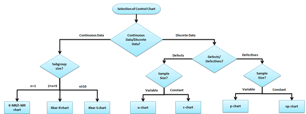
Flowchart for selecting a control chart: continuous data routes by subgroup size to I-MR (n=1), Xbar-R (2 to 8), or Xbar-S (9 or more); discrete data routes to u, c, p, or np charts depending on whether defects or defectives are counted and whether sample size is variable or constant.
Control chart Selection

The X-bar R chart is used to monitor the process performance of continuous data. You can also use it to collect data from subgroups at set time periods. It is actually two plots to monitor the process mean and the process variation over time and is an example of statistical process control. These combination charts help to understand the stability of processes and detect special-cause variation.

The cumulative sum (CUSUM) and the exponentially weighted moving average (EWMA) charts also monitor the process’s mean, but the primary difference is unlike the X bar chart. They consider the previous value means at each point.

X Bar R Control Chart Definitions

X bar chart: The mean or average change in a process over time from subgroup values. The control limits on the X̄ consider the sample’s mean and center.

R chart: The range of the process over time from subgroup values. This monitors the spread of the process over time.

Notation Used in X-bar R Charts

  • m = Number of subgroups
  • n = Number of observations per subgroup
  • X̄ = Mean of one subgroup
  • X̄̄ = Grand mean (average of all X̄ values)
  • R = Range of one subgroup
  • R̄ = Average range (average of all R values)

For example, if you measure 5 parts each day for 25 days:

  • n = 5
  • m = 25

Use X Bar R Control Charts When:

  • Even a very stable process may have some minor variations which cause instability. An X-bar R chart will help identify these variations over time.
  • When the data is assumed to be normally distributed.
  • An X-bar R chart is for a subgroup size of more than one (for an I-MR chart, the subgroup size is one only), and it is generally used when rationally collecting measurements in a subgroup size between two and ten observations.
  • The X Bar S Control chart should be considered once the subgroup size reaches roughly 9 or more; some references cite 10 as the cutoff, but around 9 is where the sample standard deviation becomes a more efficient estimator of variation than the range.
  • When the collected data is continuous (i.e., Length, Weight), it captures data in time order.

How to Interpret the X Bar R Control Charts

  • To correctly interpret an X-bar R chart, always examine the R chart first.
  • The X bar chart controls limits derived from the R bar (average range) values. If the R chart’s values are out of control, the X bar chart control limits are inaccurate.
  • If the points in the R chart are out of control, stop the process. Identify the special cause and address the issue. Then, remove those subgroups from the calculations.
  • Once the R bar chart is in control, review the X bar chart and interpret the points against the control limits.
  • All the points must be interpreted against the control limits but not specification limits. The customer or management provides specification limits, whereas control limits are derived from the average and range values of the subgroups.
  • Process capability studies can only be performed after the X bar and R chart values are within the control limits. They are not necessary for an unstable process.

Steps to follow for X bar R chart

The objective of the chart and subgroup size

  • Determine the aim of the chart and choose the essential variables.
  • Choose the appropriate subgroup size and the sampling frequency.
  • Collect a minimum of 20 to 25 sets of samples in the time sequence.

Example: In the manufacturing industry, plate thickness is one of the CTQ factors. During the Measure phase, the project team performed the process capability study and identified that the process was not capable (less than two sigmas). In the Analyze phase, they collected 20 sets of plate thickness samples with a subgroup size of 4.
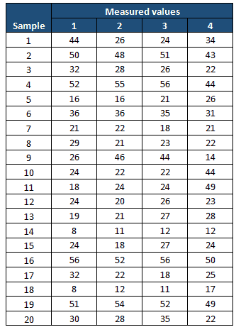
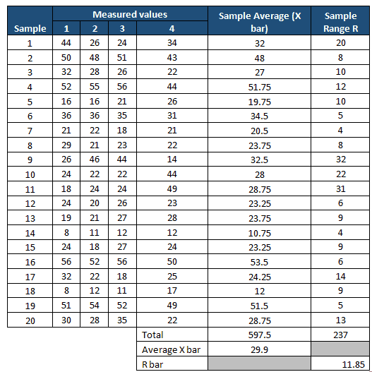
Compute X̄ and R values.

  • Measure the average of each subgroup, i.e., X-bar, and then compute the grand average of all X-bar values. This will be the center line for the X-bar chart.
  • Compute the range of each subgroup, i.e., Range, then measure the grand averages of all range values, i.e., R bar. This will be the center line for the R chart.
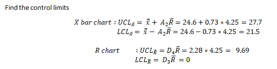
Determine the Control Limits

  • The first set of subgroups determines the process mean and standard deviation. These values are to be considered for creating control limits for both ranges and the mean of each subgroup.
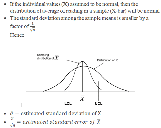
  • The process is to be under control in the early phase of production. If any of the points are out of control during the initial phase, you must identify any special causes. Also, you should remove the subgroup before the calculation.
  • Sometimes, having a few points out of control on the x-bar portion would also be good in the initial phase. Otherwise, if all the values are within the control limits, it may be because of the slop in the measurement system, and the team won’t focus on it. Identify the appropriate Measurement System Evaluation (MSE).
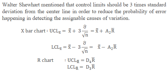
  • Where
    • X is the individual value (data)
    • n is the sample size (subgroup size)
    • X̄ is the average reading in a sample
    • R is the Range, in other words, the difference between the largest and smallest value in each sample.
    • R-bar is the average of all the ranges.
    • UCL is the Upper control limit
    • LCL is the Lower control limit

X bar chart control limits:
UCL = X̄̄ + A₂ × R̄
LCL = X̄̄ − A₂ × R̄

R chart control limits:
UCL = D₄ × R̄
LCL = D₃ × R̄

Where A₂, D₃, and D₄ are control chart constants that depend on the subgroup size n; see the constants table below. Let m represent the number of subgroups collected and n the number of observations per subgroup.

The control chart constants below are the approximate values used to measure the control limits for the X-bar R chart and other control charts based on subgroup size.
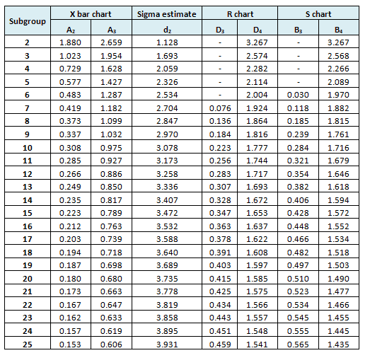
Control chart constants table showing A2, A3, d2, D3, D4, B3, and B4 by subgroup size for X-bar, R, and S charts
Control Chart Constants
Subgroup size (n)A2A3d2D3D4B3B4
21.8802.6591.128–3.267–3.267
31.0231.9541.693–2.574–2.568
40.7291.6282.059–2.282–2.266
50.5771.4272.326–2.114–2.089
60.4831.2872.534–2.0040.0301.970
70.4191.1822.7040.0761.9240.1181.882
80.3731.0992.8470.1361.8640.1851.815
90.3371.0322.9700.1841.8160.2391.761
100.3080.9753.0780.2231.7770.2841.716
110.2850.9273.1730.2561.7440.3211.679
120.2660.8863.2580.2831.7170.3541.646
130.2490.8503.3360.3071.6930.3821.618
140.2350.8173.4070.3281.6720.4061.594
150.2230.7893.4720.3471.6530.4281.572
160.2120.7633.5320.3631.6370.4481.552
170.2030.7393.5880.3781.6220.4661.534
180.1940.7183.6400.3911.6080.4821.518
190.1870.6983.6890.4031.5970.4971.503
200.1800.6803.7350.4151.5850.5101.490
210.1730.6633.7780.4251.5750.5231.477
220.1670.6473.8190.4341.5660.5341.466
230.1620.6333.8580.4431.5570.5451.455
240.1570.6193.8950.4511.5480.5551.445
250.1530.6063.9310.4591.5410.5651.435
Control chart constants (A2, A3, d2, D3, D4, B3, B4) by subgroup size, for X-bar, R, and S charts. Matches the table shown above.

Refer to common factors for various control charts.

Example cont: In the above example, n=4
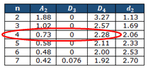
Control chart constants table with the subgroup size n=4 row highlighted: A2=0.73, D3=0, D4=2.28, d2=2.06
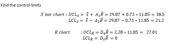
Worked control limit calculations for the plate thickness example: X-bar chart UCL=38.5, LCL=21.2; R chart UCL=27.01, LCL=0, using grand mean 29.87 and R-bar 11.85

Interpret X bar and R chart

  • Plot both the X bar and R chart and identify the assignable causes

Example Cont: Use the above values and plot the X bar and Range chart
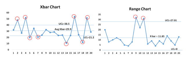
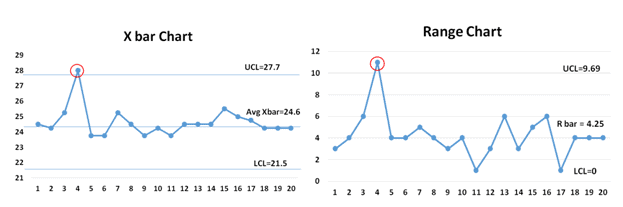
X-bar chart and Range chart for the plate thickness example, with 20 subgroups plotted against the control limits; points outside the control limits are circled in red to show out-of-control conditions
Red circles mark subgroups outside the control limits, both charts share the same 20 subgroups.

From both the X-bar and R charts, it is evident that most of the values are out of control; hence, the process is not stable.

Monitor the process after improvement.

  • Once the process stabilizes and control limits are in place, monitor the process performance over a set period.

Example cont: Control Phase: Once the process is improved and matured, the team identifies the X-bar R chart as one of the control methods in the Control plan, which is used to monitor process performance over time.

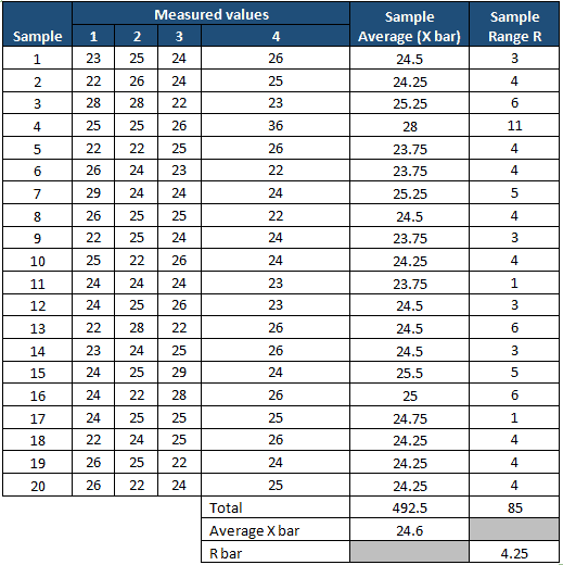
The following are the measurement values in the Control phase of the project.
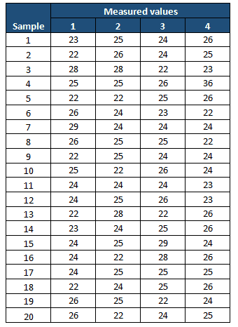
Compute X-bar and Range
X Bar R Control Charts

Both the X-bar and R charts clearly show that the process is almost stable. During the initial phase, one value is out of control, so the team has to perform a root cause analysis for the special cause. It also seems that the process is smoothing out from data set number 16. If that continued, the chart would need new control limits from that point.

  • After the process is stabilized, even if any point goes out of the control limits, it indicates an assignable cause that needs to be addressed. This is an ongoing process to monitor process performance.

https://www.youtube.com/watch?v=djEMQLS7VCc

X-bar R charts are for continuous (variable) data. If you are working with attribute data instead, see the P chart (proportion of defective units) or the NP chart (number of defective units). For a deeper look at what these control limits mean for meeting customer requirements, see Process Capability & Performance (Pp, Ppk, Cp, Cpk).

Important notes

  • A process that is “in control” means that the process is stable and predictable.
  • Just because a process is stable does not mean it has a zero-defect process.
  • Remember NEVER to put specifications on any control chart.
  • The points on the chart are comprised of averages, not individuals. Specification limits are based on individuals, not averages.
  • The operator might be prone to not reacting to a point that is out of control when the point is within the specification limits.
  • X bar R chart helps to avoid unnecessary adjustments in the process.

  X Bar R Control Chart Videos

When you’re ready, there are a few ways I can help:

First, join 12,000+ other Six Sigma professionals by subscribing to my email newsletter. A short read every Monday to start your work week off correctly. Always free.

* * *

If you’re looking to pass your Six Sigma Green Belt or Black Belt exams, I’d recommend starting with my affordable study guide:

1)→ 🟢Pass Your Six Sigma Green Belt: a study guide organized by the exam Body of Knowledge, 1,000+ practice questions with detailed answer explanations, and 8 full-length mock exams

2)→ ⚫Pass Your Six Sigma Black Belt: the full Black Belt Body of Knowledge, 2,000+ practice questions with detailed answer explanations, and 8 full-length mock exams

You’ve spent so much effort learning Lean Six Sigma. Why leave passing your certification exam up to chance? This comprehensive study guide offers 1,000+ exam-like questions for Green Belts (2,000+ for Black Belts) with full answer walkthroughs, access to instructors, detailed study material, and more.

​ Thousands have used this system to prepare. Join them here. 
Linear Regression

Linear regression is a statistical technique used to estimate the mathematical relationship between a dependent variable (usually denoted as Y) and an independent variable (usually denoted as X). In other words, predict the change in the dependent variable according to the change in the independent variable.

  • Dependent variable or Criterion variable: That is the variable for which we wish to make a prediction.
  • Independent variable or Predictor variable: The variable used to explain the dependent variable.

When to Use Linear Regression

In simple linear regression, there is only one independent variable that is used to predict a single dependent variable. Whereas in multiple linear regression, we use more than one independent variable to predict a single dependent variable. In fact, the basic difference between simple and multiple regression is in the presence of explanatory variables.

For example, compare the crop yield rate against the rainfall rate in a season.

Notes about Linear Regression

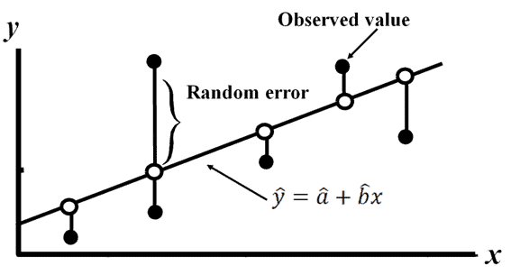
The first step of linear regression is to test the linearity assumption. This can be performed by plotting the values in a graph known as a scatter plot to observe the relationship between the dependent and independent variables. If the data is exponentially scattered, then there is no point in creating the regression equation.

Draw the line which covers the majority of the points; furthermore, we can consider this line as the “best fit” line

The mathematical equation of the line is y=a+bx+ε.

Where:

  • b: Slope of the line
  • a: y-intercept when x=0
  • Random error (ε-Epsilon): The difference between an observed value of y and the mean value of y for a given value of x.
Linear Regression

Assumption of Linear regression

  • Linear relationship between the dependent and independent variable.
  • All variables of regression to be multivariate normal.
  • Particularly there is no or little multicollinearity in the data.
  • Response variable is continuous, and also residuals are almost the same throughout the regression line.

The method of Least Squares

The method of least squares is a standard approach in regression analysis to determine the best-fit line for a given data. It basically provides a visual relationship between the given data points.

In general, the dependent variables are demonstrated on the y-axis, while the independent variables are demonstrated on the x-axis. The least square method determines the position of a straight line, which we also call a trend line or the equation of the line. This straight line is also known as the best-fit line.

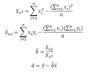
The least square method means that the overall solution minimizes the sum of squares of the errors made in the results of every single equation. For instance, we can use them to find the values of the coefficients a and b.

We can compute the least-square estimator of a and b as follows:

Linear Regression

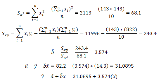
Compute â and b̂ values and then substitute these values into the equation of a line to obtain the least squares prediction equation or regression line.

Linear Regression example in DMAIC

Example: Linear Regression is specifically used in Analyze phase of DMAIC to estimate the mathematical relationship between a dependent variable and an independent variable.

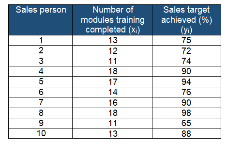
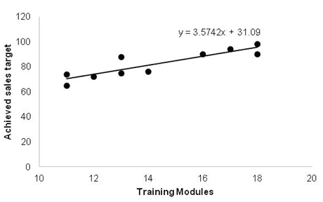
A passenger vehicle manufacturer is reviewing the 10 salespersons’ training records. In fact, their main aim is to compare the salesperson’s achieved target (in %) with the number of sales module trainings completed.

Compute the least square prediction equation or regression line.

Linear Regression

Furthermore, predict y for a given value of x by substitution into the prediction equation. For example, If a salesperson completes 15 training modules, then the predicted achieved target sales would be:

ŷ = 31.09+3.5742(15)= 84.7019=84.7%

Estimate the variability of random errors

Referring the mathematical equation of the line is y=a+bx+ε, and also the least square line is:

Linear Regression

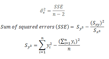
A random error (Є) affects the error of prediction. Hence, the variability of the random errors (σε2) is the key parameter while predicting by the least squares line.

Estimate variability of the random error σε2

Linear Regression

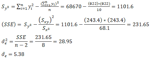
Example: From the above data, compute the variability of the random errors:

Linear Regression

From the above calculation, σ̂Є is 5.38. Thus, most of the points will fall within ±1.96 σ̂Є i.e 10.54 of the line. Hence, approx 95% of the values should be in this region. Moreover, from the above graph, it is clearly evident that all the values are within ±10.54 of the line.

Test of the slope coefficient

If we set b equal to 0, then we can test whether or not the existence of a significant relationship between the dependent and independent variables. If b is not equal to 0 there is a linear relationship. The null and alternative hypotheses are:

  • The null hypothesis H0: b=0
  • The alternative hypothesis H1:  b≠0

Degrees of freedom = n-2

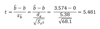
Example:  From the above data determine if the slope results are significant at a 95% confidence level.

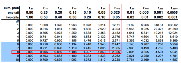
Determine the critical values of t for 8 degrees of freedom at a 95% confidence level.

t0.025, 8  = -2.306 and 2.306

The calculated t-value is 5.481, which is not in between -2.306 and 2.306. We can reject the null hypothesis if the t-value is greater than 2.306 or less than -2.306. 

In this case, we can reject the null hypothesis and conclude that b≠0 and there is a linear relationship between the dependent and independent variables.

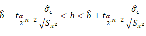
Confidence interval estimate for the slop b

The confidence interval estimate for the slope b is:

Example: from the above data, compute the confidence interval around the slope of the line:

2.0707<b<5.07

Correlation Coefficient

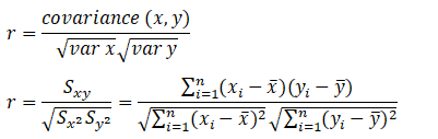
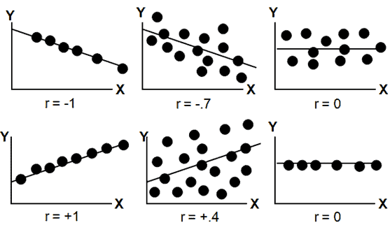
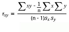
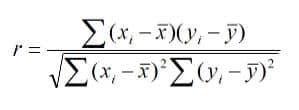
The linear correlation coefficient r measures the strength of the linear relationship between a sample’s paired x and y values.

Pearson’s Correlation Coefficient

Linear Regression

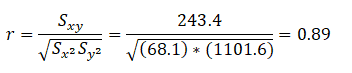
Example: From the above data, find the correlation coefficient:

Note that -1≤ r ≤ +1:

  • The line slopes upward to the right when r indicates a positive value.
  • The line slopes downward and to the right when r indicates a negative value.
  • A value closer to 1, indicates the stronger positive linear relationship.
  • A value closer to -1, indicates the stronger negative linear relationship.
  • When r=0 implies no linear correlation.
Linear Regression

How is correlation analysis used to compare bivariate data?

The Measure of central tendency, variance, or spread, summarizes a single variable. It does this by providing important information about its distribution as can be seen below in the example. Often, more than one variable is collected in a study or experiment. The resulting data are bivariate when two variables are measured on a single experiment unit. For example, job satisfaction is stratified by income.

In most instances, in bivariate data, it determines that one variable influences the other variable. Furthermore, the quantities from these two variables are often represented using scatter plots to explore the relation between the two variables.

Bivariate data can be described with graphs and numerical measures depending on the data type. If one or both variables are qualitative, use a pie chart or bar chart to see the relationship between variables. For example, compare the relationship between opinion and gender. If the two variables are quantitative, use the scatter plot. The Correlation Coefficient is often used in comparing bivariate data.

Example:

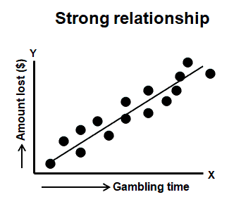
Correlation between the amount of time spent in a Casino (independent variable) and the amount ($) lost (dependent variable).

correlation coefficient

The correlation coefficient varies between -1 and +1. Values approaching -1 or +1 indicate a strong correlation (negative or positive), and values close to 0 indicate little or no correlation between x and y.

Sample Correlation Coefficient

Correlation does not mean causation.

A positive correlation can be either good news or bad news.

A negative correlation is not necessarily bad news. It merely means that as the independent variable increases, the dependent variable tends to decrease.

r = 0; does not indicate the absence of a relationship, a curvilinear pattern may exist; r=-0.76 has the same predictive power as r = +0.76.

Correlation Coefficient Videos

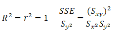
Coefficient of determination (R2)

The coefficient of determination is the proportion of the explained variation divided by the total variation when linear regression is performed.

Linear Regression

r2 lines in the interval of 0≤ r2 ≤1.

Example: Now that we have the above data, compute the coefficient of determination.

We can say that 79% of the variation in the overall number of training modules completed explains the variation in the sales targets.

Residual Analysis: “Because a linear regression model is not always appropriate for the data, you should assess the appropriateness of the model by defining residuals and examining residual plots.”

Linear Regression Additional Videos

When you’re ready, there are a few ways I can help:

First, join 12,000+ other Six Sigma professionals by subscribing to my email newsletter. A short read every Monday to start your work week off correctly. Always free.

* * *

If you’re looking to pass your Six Sigma Green Belt or Black Belt exams, I’d recommend starting with my affordable study guide:

1)→ 🟢Pass Your Six Sigma Green Belt: a study guide organized by the exam Body of Knowledge, 1,000+ practice questions with detailed answer explanations, and 8 full-length mock exams

2)→ ⚫Pass Your Six Sigma Black Belt: the full Black Belt Body of Knowledge, 2,000+ practice questions with detailed answer explanations, and 8 full-length mock exams

You’ve spent so much effort learning Lean Six Sigma. Why leave passing your certification exam up to chance? This comprehensive study guide offers 1,000+ exam-like questions for Green Belts (2,000+ for Black Belts) with full answer walkthroughs, access to instructors, detailed study material, and more.

​ Thousands have used this system to prepare. Join them here. 

ANOVA Analysis of Variation

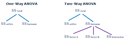
Analysis of Variance (ANOVA) is a parametric statistical technique used to compare data sets. This technique was invented by R.A. Fisher; hence, it is also referred to as Fisher’s ANOVA. It is similar to techniques such as t-test and z-test to compare means and also the relative variance between them.

Similarly, a t-test can be used to compare two sample means. What if we want to compare more than two means? Analysis of variance (ANOVA) is best applied where more than 2 populations or samples are meant to be compared.

It is used to test the statistical significance of the relationship between a dependent variable (“Y”) and single or multiple independent variables (“X’s”).

Types of ANOVA

  • One-way
    • Measures single factor from multiple sources
    • Uses only one technician / one measurer
  • Two-way (without replicates)
    • Measures 2 factors
    • Uses only one technician (unless technicians are one of the factors)
  • Two-way (with replications)
    • Measures 2 factors but has multiple repetitions of each combination.
    • Uses only one technician (unless the technicians are one of the factors)

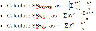
ANOVA Sum of Squares Correction Factor

  • Grand total of all runs (G) = ΣX
  • N= Total number of runs
  • Correction factor (CF)= (ΣX)2 /N = (G)2 /N

Terms used in ANOVA

  • Degrees of Freedom (df): The number of independent conclusions that can be drawn from the data. 
  • SSFactor: It measures the variation of each group’s mean to the overall mean across all groups. 
  • SSError: It measures the variation of each observation within each factor level to the mean of the level. 
  • Main effect: A main effect is an effect where the performance of one variable is considered in isolation by neglecting other variables in the study.
  • Interaction: An interaction effect occurs where the effect of one variable is different across levels of one or more other variables.
  • Mean Square Error (MSE): The mean square of the error (MSE) is divided by the sum of squares of the residual error by the degrees of freedom.
  • F-test Statistic: The null hypothesis that the category means are equal in the population is tested by F Statistic based on the ratio of mean square related to X and mean square related to the error.
  • P-value: It is the smallest level of significance that would lead to rejection of the null hypothesis (Ho). If α = 0.05 and the p-value ≤ 0.05, then reject the null hypothesis. Similarly if the p-value > 0.05, then fail to reject the null hypothesis.

https://youtu.be/x6F9uvaviEc

Analysis of Variance (ANOVA) has three types:

  • One-way analysis
  • Two-way analysis
  • K-way analysis: K-Way ANOVA can be two-way ANOVA or three-way ANOVA, or multiple ANOVA

One way ANOVA

One-way ANOVA (one-way analysis of variance) is a statistical method to compare the means of two or more populations.

Assumptions of One-way ANOVA

  • The sample data drawn from k populations are unbiased and representative.
  • The data of k populations are continuous.
  • The data of k populations are normally distributed.
  • The variation within each factor or factor treatment combination is the same; hence, it is also called homogeneity of variance.
  • Finally, the variances of k populations are equal.

Steps for Computing one-way ANOVA:

  • Establish the hypotheses. H0: µ1= µ2= µ3 and H1: At least one group means differs from the others.
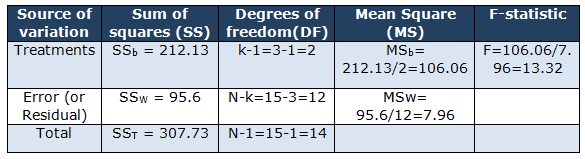
  • In ANOVA, the total variance is subdivided into two independent variances: the variance due to the treatment and the variance due to random error.
  • SST = SSb + SSw 
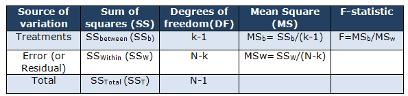
  • Calculate the ANOVA table with degrees of freedom (df), and calculate the group’s error and total sum of squares.
  • SSb= sum of squares between treatments
  • SSw= sum of squares due to error
  • MSb= mean square for treatments
  • MSW= mean square for error
  • SST= total sum of squares
  • T= number of treatment levels
  • n= number of runs at a particular level
  • N= total number of runs
  • F= the calculation of the F Statistic with k-1, and N-k is the degrees of freedom.
  • Determine the critical value. F critical value from the F distribution table.
  • Finally, Draw the statistical conclusion. If Fcalc< Fcritical, fail to reject the null hypothesis, and if Fcalc > Fcritical, reject the null hypothesis.

Example of One-Way ANOVA

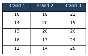
A car manufacturer planned to conduct tests to determine the performance of 3 different brands of 12V batteries, so he selected five batteries from each brand and discharged them under controlled conditions. Assuming the lifetime of batteries is normally distributed at a 95% confidence level. The hypothesis is that the three brands have no difference in lifetime.

H0: µ1= µ2= µ3

H1: At least one of the brands mean life is different from the others.

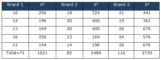
k = 3, n = 5, N = 15, T1 = 71, T2 = 85, and T3 = 116, and G = 272 ΣX2= 1021 + 1489 + 2730 = 5240

Correction factor (CF) = (ΣX)2 /N = (G)2 /N = (272)2/15

One-Way ANOVA Excel Download

Unlock Additional Members-only Content!

To unlock additional content, please upgrade now to a full membership.
Upgrade to a Full Membership
If you are a member, you can log in here.

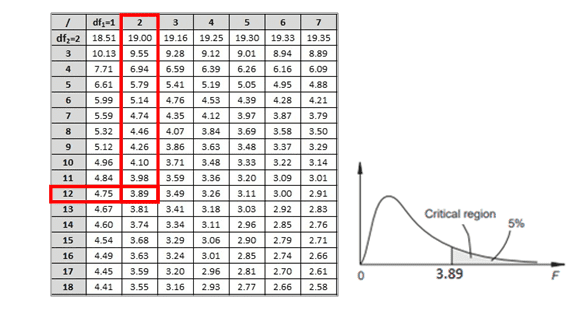
For α = .05, the critical value for F with d.f. (2, 12) is 3.89.

Fcalc > Fcritical; hence, we may have to reject the null hypothesis.

The calculated value does lie in the critical region. Therefore, there is evidence, at the 5% significance level, that the mean lifetime of the three brands’ batteries differs.

Example One-Way ANOVA

Three different brands of chlorine are used at a local pool throughout the summer. Initially, they used one brand. As one brand’s four-week supply runs out, the staff begins using the next brand of chlorine. Management is interested in determining if the different brands significantly affect the ability to maintain safe pH levels. Once the previous brand is no longer present in any measurable amount, the pH levels for each brand are collected through random sampling. Is there a significant difference between the three brands of chlorine? Test at the 5% significance level. Complete the ANOVA table (except the p-value) manually.

One way ANOVA
One way ANOVA 

Two way ANOVA

Two-way ANOVA performs an analysis of variance for testing the equality of population means when the classification of treatments is by two categorical (independent) variables or factors.

Assumptions of Two-way ANOVA

  • The cells contain independent samples
  • Two main effects and an interaction
  • The populations should have equal variance
  • Balanced data and fixed factors

Steps for Computing Two-way ANOVA:

  • Establish the hypotheses: The null hypotheses for each of the sets are given below:
  • The population means of the first factor are equal. This is like the one-way ANOVA for the row factor.
  • The population means of the second factor are equal. This is like the one-way ANOVA for the column factor.
  • There is no interaction between the two factors. This is similar to performing a test for independence with contingency tables.
  • Calculate the test statistic and rejection region.
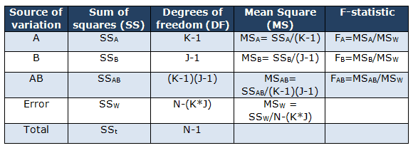
  • Calculate SSAB(Interaction) as= SSt-SSw-SSA-SSB
    • a: number of levels in factor A
    • b: number of levels in factor B
    • r: total number of trials
    • Xi..: mean of the i th factor level of factor A
    • X…: overall mean of all observations
    • X.j.: mean of the j th factor level of factor B
    • Xij.: mean of observations at the i th level of factor A and the j th level of factor B
  • Calculate the ANOVA table with degrees of freedom (df) and F value as shown below.
  • Determine the critical value. Remember, F(critical) is from the F distribution table.
  • Finally, Draw the statistical conclusion. If Fcalc< Fcritica,l fail to reject the null hypothesis, and if Fcalc > Fcritical, reject the null hypothesis.

Example:

A researcher experimented to check the effectiveness of the coating. A new coating was applied to two different materials, and research was conducted at two different laboratories. For instance, each laboratory tested five samples from each treated material. Find the results from the table below:

For α = .05, the critical value for F with d.f. (1, 16) is 4.49.

There appears to be both Laboratory and Material Fcalc > Fcritical; hence, we reject the null hypothesis. But for the interaction, Fcalc< Fcritical, hence, fails to reject the null hypothesis.

https://www.youtube.com/watch?v=7vLp8MDwgcE&feature=youtu.be

Multivariate Analysis of Variance (MANOVA)

Multivariate analysis of variance (MANOVA) is an ANOVA with several dependent variables. That is to say, ANOVA tests for the difference in means between two or more groups, while MANOVA tests for the difference in two or more vectors of means.

MANOVA examines the dependence relationship between dependent measures across a set of groups. Moreover, this analysis is used in experimental design, and the hypothesized relationship between dependent measures is usually used.

Assumptions of MANOVA

  • The response variables are continuous.
  • The residuals follow the multivariate-normal probability distribution with means equal to zero.
  • The variance-covariance matrices of each group of residuals are equal.
  • The individuals are independent.

Interestingly, in addition to detecting differences in the average values, it also detects differences in correlations among the dependent variables between the different levels of the independent variable.

Benefits of MANOVA

There are various advantages of MANOVA over ANOVA.

  • Study any interaction between the factors.
  • Study two or more factors simultaneously to increase the model’s efficiency.
  • MANOVA reduces the chances of alpha risk.
  • Less residual variation in the model when more factors are in the study.

Additional Resources for ANOVA

http://psychnut.com/statistics/even-more-about-1-way-anova/

https://www.technologynetworks.com/informatics/articles/one-way-vs-two-way-anova-definition-differences-assumptions-and-hypotheses-306553

http://oak.ucc.nau.edu/rh232/courses/EPS525/Handouts/Understanding%20the%20One-way%20ANOVA.pdf

Six Sigma Black Belt Certification ANOVA Questions:

Question: To assess the significance of factors in either a fractional or a full-factorial experiment structure, a black belt can be used: (Taken from ASQ sample Black Belt exam.)

(A) analysis of variance (ANOVA)
(B) fault tree analysis (FTA)
(C) failure mode and effects analysis (FMEA)
(D) evolutionary operation (EVOP)

Answer: 

Unlock Additional Members-only Content!

To unlock additional content, please upgrade now to a full membership.
Upgrade to a Full Membership
If you are a member, you can log in here.

When you’re ready, there are a few ways I can help:

First, join 12,000+ other Six Sigma professionals by subscribing to my email newsletter. A short read every Monday to start your work week off correctly. Always free.

* * *

If you’re looking to pass your Six Sigma Green Belt or Black Belt exams, I’d recommend starting with my affordable study guide:

1)→ 🟢Pass Your Six Sigma Green Belt: a study guide organized by the exam Body of Knowledge, 1,000+ practice questions with detailed answer explanations, and 8 full-length mock exams

2)→ ⚫Pass Your Six Sigma Black Belt: the full Black Belt Body of Knowledge, 2,000+ practice questions with detailed answer explanations, and 8 full-length mock exams

You’ve spent so much effort learning Lean Six Sigma. Why leave passing your certification exam up to chance? This comprehensive study guide offers 1,000+ exam-like questions for Green Belts (2,000+ for Black Belts) with full answer walkthroughs, access to instructors, detailed study material, and more.

​ Thousands have used this system to prepare. Join them here. 

One Sample T Hypothesis Test (Student’s T-Test)

One Sample T-Tests (Student’s T-Test) are used to resolve Hypothesis tests around comparing process means. The underlying chart makes use of the T-distribution.

Student’s T-distribution uses the T-distribution and is used for finding confidence intervals for the population mean when the sample size is less than 30, and the population Standard Deviation is unknown. 

What is a One Sample T Hypothesis Test?

The One Sample T Hypothesis Test (Student’s T-Test) allows one to compare the (small) population mean to some hypothesized value or one sample mean to determine if they are significantly different.

For example, if we know the average weight of chickens on a farm is 3lb, and compare the average weight of sample black hens to the population mean value.

When Would You Use a One Sample T Hypothesis Test?

One sample T-Test is a type of parametric test because the assumption is samples are randomly distributed. It tests whether the sample mean is significantly different than a population mean when the standard deviation of the population is unknown. Hence, a T-Test is used when the population standard deviation is unknown, and the sample size is below 30. Otherwise, use Z-test (for known variance).

Assumptions of One Sample T Hypothesis Test

  • Data is continuous and quantitative at the scale level (in other words, data in ratio or interval).
  • The sample should be randomly selected from the population.
  • Samples are independent of each other.
  • Data should follow a normal probability distribution.
  • Assumes it doesn’t have extreme outliers in the dependent variable.

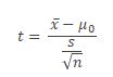
One Sample T Hypothesis test formula

One Sample T Hypothesis Test (Student's T Test)
  • Where
    • x̅ is observed sample mean
    • μ0 is the population mean
    • s is the sample Standard Deviation
    • n is the number of observations in the sample

Steps to Calculate One Sample T Hypothesis Test

  • State the claim of the test and determine the Null Hypothesis and Alternative Hypothesis.
  • Determine the level of significance.
  • Calculate degrees of freedom.
  • Find the critical value.
  • Calculate the test statistics.
  • Make a decision, the Null Hypothesis will be rejected if the test statistic is in the rejection region.
  • Finally, interpret the decision in the context of the original claim.

One Sample T-Test Hypothesis

Null Hypothesis (H0): The difference between the population mean and the hypothesized value is equal to zero.

Alternative Hypothesis (H1):

  • The population mean is not equal to the hypothesized value (Two-tailed).
  • The population mean is greater than hypothesized value (Upper-tailed).
  • The population mean is less than hypothesized value (Lower-tailed).

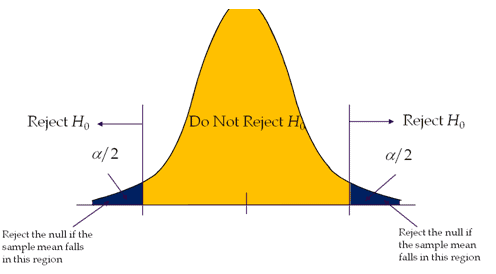
Two-Tailed T Test

A hypothesis test is performed if the population parameter is suspected to be different from the Null Hypothesis’s assumed parameter.

  • H0: μ=μ0
  • H1: μ≠μ0.
One Sample T Hypothesis Test (Student's T Test)

Right-tailed or Upper-tailed test

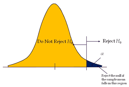
The Right-tailed test is also called the Upper-tail test. A hypothesis test is performed if the population parameter is suspected to be greater than the assumed parameter of the Null Hypothesis.

  • H0: μ≤μ0
  • H1: μ>μ0
One Sample T Hypothesis Test (Student's T Test)

Left-tailed test or Lower-tailed test

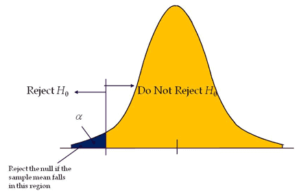
The Left-tailed test is also known as a Lower-tail test. A hypothesis test is performed if the population parameter is suspected to be less than the assumed parameter of the Null Hypothesis.

  • H0: μ≥μ0
  • H1: μ<μ0
One Sample T Hypothesis Test (Student's T Test)

Example of a One-Sample T Hypothesis Test in a DMAIC Project

One Sample T-Tests are mostly carried out in Analyze phase of DMAIC to check the significant differences between the population mean and the sample means, while paired T-Tests can be done in the Measure phase to review before and after process improvement (see below example for more details).

Example of Two-Tailed Test

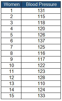
Example: According to the American Health Association, a pregnant woman’s average blood pressure is 120 mm Hg. Collected 15 random samples from pregnant women to check whether the sample blood pressure differs from accepted standard blood pressure.

  • Null Hypothesis: H0: μ=120
  • Alternative Hypothesis: H1: μ≠120

Significance level: α=0.05

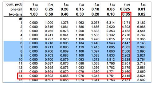
Degrees of freedom: 15 – 1 = 14

Calculate the critical value

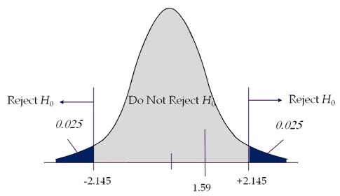
If the calculated t value is less than -2.145 or greater than 2.145, then reject the Null Hypothesis.

Test Statistics

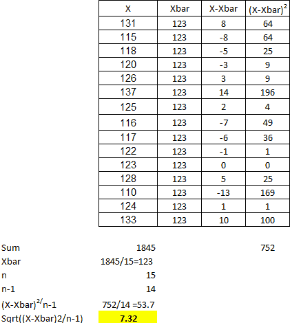
  • x̅ = 123
  • μ0 = 120
One Sample T Hypothesis Test (Student's T Test)

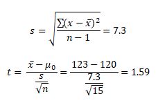
Interpret the results: Compare t calc to t critical. In hypothesis testing, a critical value is a point on the test distribution compared to the test statistic to determine whether to reject the Null Hypothesis. The calculated t-statistic value is less than the critical value; hence we failed to reject Null Hypothesis.

One Sample T Two-Tailed Test Excel Template

Unlock Additional Members-only Content!

To unlock additional content, please upgrade now to a full membership.
Upgrade to a Full Membership
If you are a member, you can log in here.

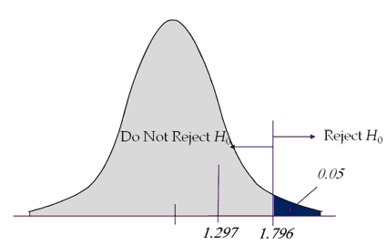
Right-tailed test

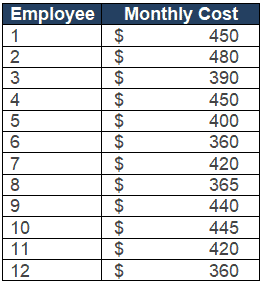
Example: A software start-up company plans to introduce company transportation based on the town hall meeting’s feedback. The admin manager randomly collected 12 employees’ spending on public transportation for the month. With a 95% confidence level, is there any evidence that the population mean is above $400?

  • Null Hypothesis: H0: μ≤400
  • Alternative Hypothesis: H1: μ>400

Significance level: α = 0.05

Sample size n =12

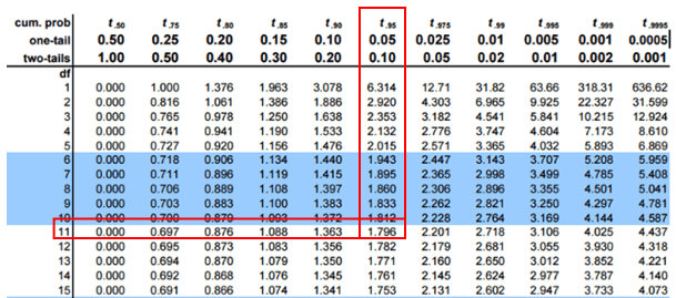
Degrees of freedom: 12 – 1 = 11

Calculate the critical value

One Sample T Hypothesis Test (Student's T Test)

If the calculated t value is greater than 1.796, then, reject the Null Hypothesis.

Calculate the Test Statistics

  • Sum of all samples =4980
  • x̅ = Σx/n = 4980 / 12=415
  • Σ(X-X̅)2 = 17650
  • Σ(X-X̅)2 /n-1 = 1604.5
  • Standard Deviations = √ Σ(X-X̅)2 /n-1 = 40
  • μ0 = 400
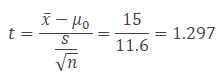
  • x̅- μ0 =15
  • s/√n = 40/√12 = 11.6

Interpret the results: Compare t calc to t critical. In hypothesis testing, a critical value is a point on the test distribution compared to the test statistic to determine whether to reject the Null Hypothesis. Since tcal value is less than t critical value and it is not in the rejection region. Hence we failed to reject the Null Hypothesis. There is no sufficient evidence to claim the population mean is above $400.

One Sample T Two-Tailed Test Excel Template

Unlock Additional Members-only Content!

To unlock additional content, please upgrade now to a full membership.
Upgrade to a Full Membership
If you are a member, you can log in here.

Left-tailed test

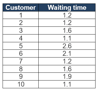
Example: The average waiting time for billing at XYZ restaurant is 1.9 minutes. The restaurant owner updated the billing software to reduce the waiting time. He randomly collected 10 customers waiting time at the billing counter. With a 95% confidence level, is there any evidence that the population’s average waiting time is less than 1.9 minutes?

  • Null Hypothesis: H0: μ≥1.9
  • Alternative Hypothesis: H1: μ<1.9

Significance level: α = 0.05

Sample size n = 10

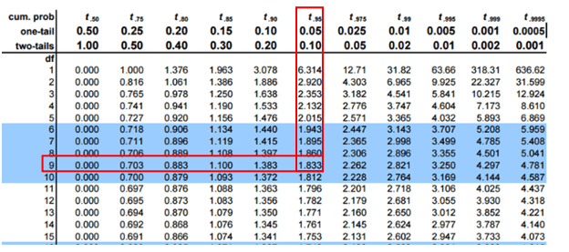
Degrees of freedom: 10 – 1 = 9

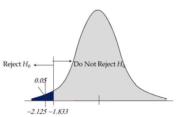
Calculate the critical value

If the calculated t value is less than -1.833, then reject the Null Hypothesis.

Calculate the test Statistics

  • Sum of all samples = 15.6
  • x̅ = Σx/n = 15.6 / 10 = 1.56
  • Σ(X-X̅)2 = 2.3
  • Σ(X-X̅)2 /n-1 = 0.3
  • Standard Deviations = √ Σ(X-X̅)2 /n-1 = 0.51
  • μ0 = 1.9
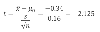
  • x̅- μ0 =-0.34
  • s/√n = 0.51 / √10 = 0.16

Interpret the results: Compare t calc to t critical. In hypothesis testing, a critical value is a point on the test distribution compared to the test statistic to determine whether to reject the null hypothesis. Since tcal value is less than the t critical value and it is in the rejection region. In other words, the absolute value of t calculated is greater than the t critical. Hence we reject the Null Hypothesis. There is sufficient evidence to claim the population mean is less than 1.9 minutes.

One Sample T Left Tailed Test Excel Template

Unlock Additional Members-only Content!

To unlock additional content, please upgrade now to a full membership.
Upgrade to a Full Membership
If you are a member, you can log in here.

One Sample T Hypothesis Test Videos

Additional One Sample T Hypothesis Test Resources

https://www.cliffsnotes.com/study-guides/statistics/univariate-inferential-tests/one-sample-t-test (One sample T-Test)

http://stattrek.com/probability-distributions/t-distribution.aspx

When you’re ready, there are a few ways I can help:

First, join 12,000+ other Six Sigma professionals by subscribing to my email newsletter. A short read every Monday to start your work week off correctly. Always free.

* * *

If you’re looking to pass your Six Sigma Green Belt or Black Belt exams, I’d recommend starting with my affordable study guide:

1)→ 🟢Pass Your Six Sigma Green Belt: a study guide organized by the exam Body of Knowledge, 1,000+ practice questions with detailed answer explanations, and 8 full-length mock exams

2)→ ⚫Pass Your Six Sigma Black Belt: the full Black Belt Body of Knowledge, 2,000+ practice questions with detailed answer explanations, and 8 full-length mock exams

You’ve spent so much effort learning Lean Six Sigma. Why leave passing your certification exam up to chance? This comprehensive study guide offers 1,000+ exam-like questions for Green Belts (2,000+ for Black Belts) with full answer walkthroughs, access to instructors, detailed study material, and more.

​ Thousands have used this system to prepare. Join them here. 
F-Test

An F-Test uses the F-distribution to determine whether two independent estimates of population variance differ significantly. It’s the tool behind ANOVA’s equality-of-means test and behind checking whether two samples come from populations with equal variance.

What is an F-Test?

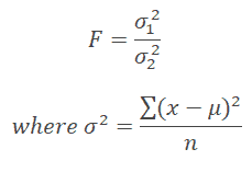
The F-test determines whether the two independent estimates of population variance differ significantly. In this case, the F-ratio is:

F ratio formula: F equals sigma-1-squared over sigma-2-squared, where population variance sigma-squared equals the sum of (x minus mu) squared, divided by n

or

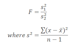
To determine whether the two samples drawn from the normal population have the same variance. In this case, the F-ratio is:

F ratio formula for two samples: F equals s-1-squared over s-2-squared, where sample variance s-squared equals the sum of (x minus x-bar) squared, divided by n minus 1

In both cases, σ12 > σ22,  S12 > S22, in other words, a larger estimate of variance always be in the numerator and a smaller estimate of variance in the denominator.

Degrees of freedom (ϑ)

  • DF of larger variance (i.e., numerator) =n1-1
  • DF of smaller variance (i.e., denominator) =n2-1

What is an F-Statistic?

F-statistic, also known as F-value, is used in ANOVA and regression analysis to identify whether the means between two populations are significantly different or not. In other words, F-statistic is the ratio of two variances (Variance is nothing but a measure of dispersion; it tells how far the data is dispersed from the mean). F-statistic accounts for corresponding degrees of freedom to estimate the population variance.

F-statistic is almost similar to t-statistic. The T-test states whether a single variable is statistically significant or not, whereas the F-test states whether a group of variables is statistically significant.

F-statistics are based on the ratio of mean squares. F-statistic is the ratio of the mean square for treatment or between groups with the Mean Square for error or within groups.

F = MS Between / MS Within

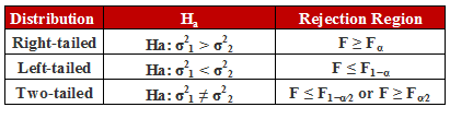
Summary table of F-test hypothesis testing by tail direction: right-tailed (Ha: sigma1-squared greater than sigma2-squared, rejection region F greater than or equal to F-alpha), left-tailed (Ha: less than, rejection region F less than or equal to F-1-minus-alpha), and two-tailed (Ha: not equal, rejection region in both tails)

If the calculated F-value is greater than the appropriate value of the F critical value (found in a table or provided in software), then the null hypothesis can be rejected. (helpful in ANOVA)

The calculated F-statistic for a known source of variation is found by dividing the mean square of the known source of variation by the mean square of the unknown source of variation.

When would you use an F-Test?

There are different types of F tests, each for a different purpose.

  • In statistics, an F-test of equality of variances is a test for the null hypothesis that two normal populations have the same variance.
  • The F-test tests the equality of several means. At the same time, ANOVA tests the equality of means.
  • F-tests for linear regression models are to test whether any of the independent variables in the multiple linear regression are significant or not. It also indicates a linear relationship between the dependent variable and at least one of the independent variables.

Steps to Conduct an F-test

  • Choose the test: Note the independent and dependent variables and assume the samples are normally distributed.
  • Calculate the F statistic and choose the highest variance in the numerator and lowest variance in the denominator with a degree of freedom (n-1).
  • Determine the statistical hypothesis.
  • State the level of significance.
  • Compute the critical F value from the F table. (use α/2 for a two-tailed test)
  • Calculate the test statistic.
  • Finally, draw the statistical conclusion. Reject the null hypothesis if the test statistic falls in the critical region.

Examples of Using an F-Test in a DMAIC Project

In the Measure and Analyze phase of DMAIC, the F-test is used to determine whether the two independent estimates of population variance differ significantly or whether the two samples drawn from the normal population have the same variance.

Using an F-Test in Hypothesis Testing

A tailed hypothesis is an assumption about a population parameter. The assumption may or may not be true. A one-tailed hypothesis tests the hypothesis where the area of rejection is only in one direction. Whereas two-tailed, the area of rejection is in two directions. The selection of one or two-tailed tests depends upon the problem.

In the F-sampling distribution, F is calculated by dividing the variance of one sample by the other sample’s variance.

For the right-tailed and two-tailed tests, keep the highest variance as the numerator and the lowest variance as the denominator. So, the numerator’s degree of freedom is the degree of freedom for the sample with the highest variance. The degree of freedom for the denominator is the degree of freedom for the sample with the lowest variance.

Right-tailed and two-tailed formula: F equals s-1-squared over s-2-squared, equal to degrees of freedom of the sample with highest variance over degrees of freedom of the sample with lowest variance

Meanwhile, for the left-tailed test, keep the lowest variance as the numerator and the highest variance as the denominator. So, the numerator’s degree of freedom is the degree of freedom for the sample with the lowest variance. The degree of freedom for the denominator is the degree of freedom for the sample with the highest variance.

Left-tailed formula: F equals s-1-squared over s-2-squared, equal to degrees of freedom of the sample with lowest variance over degrees of freedom of the sample with highest variance

Using an F-Test in Hypothesis testing: Right-tailed test

Example: A botanical research team wants to study the growth of plants using urea. The team conducted eight tests with a variance of 600 during the initial state, and after six months, six tests were conducted with a variance of 400. The experiment aims to know if there is any improvement in plant growth after six months at a 95% confidence level.

  • Degrees of freedom ϑ1 = 8 -1 = 7 (highest variance in the numerator)
  • ϑ2 = 6 – 1 = 5
  • Statistical hypothesis:
    • Null hypothesis H0: σ12≤ σ22
    • Alternative hypothesis H1: σ12>σ22
  • Since the team wants to see the improvement, it is a one-tail (right) test
  • Level of significance α= 0.05
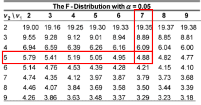
F-distribution critical value table at alpha=0.05, with row v2=5 and column v1=7 highlighted, intersecting at the critical value 4.88
  • Compute the critical F from table = 4.88
  • Reject the null hypothesis if the calculated F-value is more than or equal to 4.88
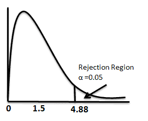
  • Calculate the F-value F= S12/ S22 =600/400= 1.5
  • Fcalc< Fcritical Hence, fail to reject the null hypothesis
F-distribution curve for the right-tailed example with the calculated F-value 1.5 marked and the critical F-value 4.88 marking the start of the rejection region at alpha=0.05
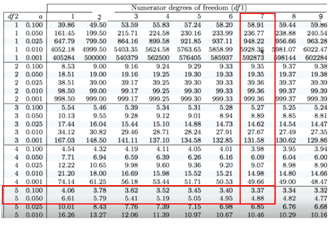
F-distribution table showing critical values across multiple alpha levels (0.100, 0.050, 0.025, 0.010, 0.001) for numerator df=7, with the row for denominator df=5 highlighted showing 3.37 at alpha=0.100 and 4.88 at alpha=0.050

p-value

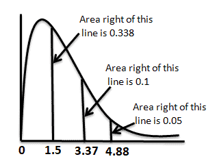
We can find F critical values from the F table that give us a certain area to the right. From the above table, the area to the right of 4.88 is 0.05, and the area to the right of 3.37 is 0.100. So, the area to the right of 1.5 from the graph must be more than 0.100. However, we can easily find the exact p-value using any statistical tool or Excel.

How to calculate p-value in Excel

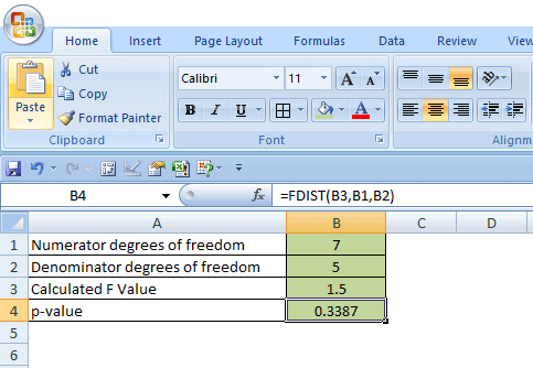
  • Enter numerator degrees of freedom in the B1 cell.
  • Then, enter the denominator degrees of freedom value in the B2 cell.
  • Enter the calculated F value in the B3 cell.
  • Now, p-value = use FDIST function in Excel. In B4 cell type =FDIST(B3, B1, B2), click on enter, and you will get the exact p-value for the right-tailed test.
Excel spreadsheet with the FDIST formula =FDIST(B3,B1,B2) entered, using numerator df=7, denominator df=5, and calculated F value 1.5, returning a p-value of 0.3387
F-distribution curve with three marked points (1.5, 3.37, 4.88) each labeled with the area to their right (0.338, 0.1, and 0.05 respectively), illustrating how the p-value 0.338 relates to the critical values

Interpret the results:

Compare f calc to f critical. In hypothesis testing, a critical value is a point on the test distribution that is compared to the test statistic to determine whether to reject the null hypothesis. Since the f cal value is less than the f critical value, it is not in the rejection region. Hence, we failed to reject the null hypothesis at a 95% confidence level.

F-Test Right-Tailed Excel Template

Unlock Additional Members-only Content!

To unlock additional content, please upgrade now to a full membership.
Upgrade to a Full Membership
If you are a member, you can log in here.

Using an F-Test in Hypothesis testing: Two-tailed test

A toy manufacturer is planning to place a bulk order for toy batteries. The quality team collected 21 samples from supplier A with a variance of 36 hours and 16 samples from supplier B with a variance of 28. At a 95% confidence level, determine if there is a difference in variance between the two suppliers.

  • Degrees of freedom ϑ1 = 21 – 1 = 20 (highest variance in the numerator)
  • ϑ2 = 16 – 1 = 15
  • Statistical hypothesis:
    • Null hypothesis H0: σ12 = σ22
    • Alternative hypothesis H1: σ12 ≠ σ22
  • Since the team wants to see if there is a difference between the two suppliers, it is a two-tailed test.
  • Level of significance α = 0.05.

α/2 = 0.025

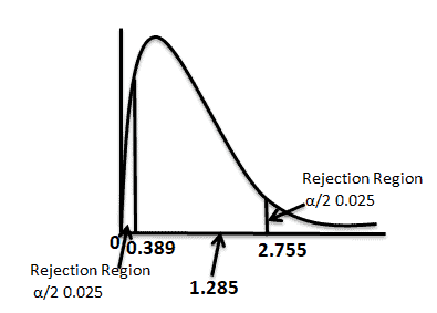
  • The critical value for the right tail F(0.025,20,15) = 2.7559.
  • The critical value for the left tail: Since it is a left tail, we must switch the degrees of freedom and then take a reciprocal of the final answer.
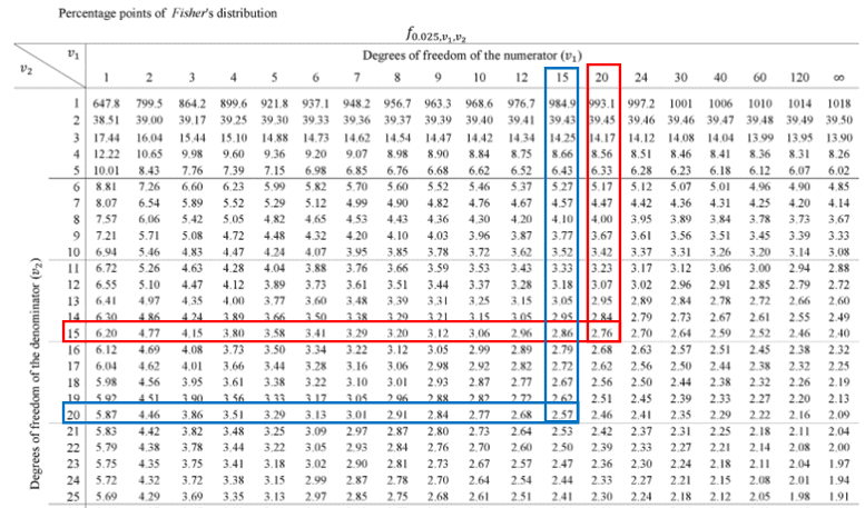
Percentage points of Fisher's F-distribution table at alpha=0.025, with the row for df2=15/df1=20 highlighted (2.76) and the reciprocal row df2=20/df1=15 highlighted (2.57), used to find the left-tail critical value
  • Reciprocal of F(0.025,15,20) = 1/F(0.025,15,20) = 1/2.57 = 0.389
  • Calculate the F value F = S12/ S22 = 36/28 = 1.285
F-distribution curve for the two-tailed example with rejection regions in both tails (each alpha/2=0.025) below 0.389 and above 2.755, and the calculated F-value 1.285 marked in the non-rejection middle region

Interpret the results:

Compare f calc to f critical. In hypothesis testing, a critical value is a point on the test distribution that is compared to the test statistic to determine whether to reject the null hypothesis. Since the f cal value does lie not lie in the rejection region, we failed to reject the null hypothesis at a 95% confidence level.

F Test Two-Tailed Excel Template

Unlock Additional Members-only Content!

To unlock additional content, please upgrade now to a full membership.
Upgrade to a Full Membership
If you are a member, you can log in here.
F-Test Sample Questions

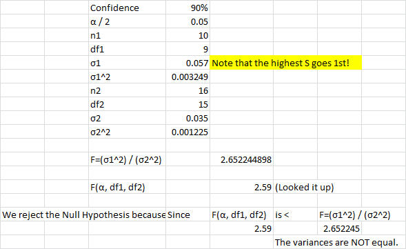
In a manufacturing facility, two Six Sigma Greenbelts monitor the process running the two stamping presses simultaneously. Each press runs the same progressive die. Student A says that he is 90% confident that the stamping presses have the same variance, while student B says the variances are different at the 90% confidence level. Which student is right? Press1: s = 0.035, n = 16 ; Press 2: s = 0.057, n = 10

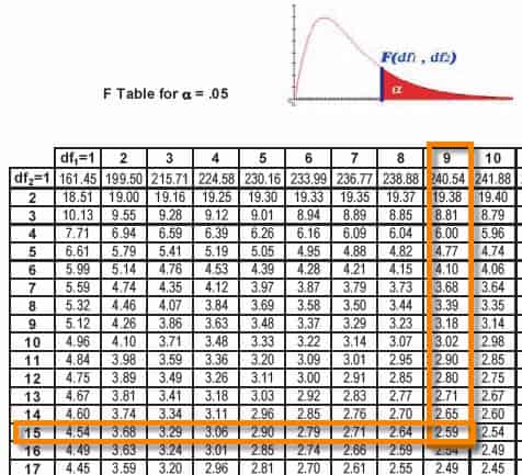
Worked solution to the stamping press sample question: 90% confidence, n1=10, df1=9, sigma1=0.057, n2=16, df2=15, sigma2=0.035, calculated F=2.652245, critical F=2.59, conclusion: reject the null hypothesis, the variances are not equal
F-distribution critical value table at alpha=0.05 used for the sample question, with row df2=15 and column df1=9 highlighted showing the critical value 2.59

Left-tailed test

XYZ is an e-commerce site that wants to test if the delivery times in Boston are less than in New York City at a 5% significance level during the Thanksgiving holidays. Twenty-eight delivery times are observed from Boston, with a variance of 38 hours. Twenty-five samples were collected from New York City with a variance of 83 hours.

  • Degrees of freedom ϑ1 = 28 – 1 = 27
  • ϑ2 = 25 – 1 = 24
  • Statistical hypothesis:
    • Null hypothesis H0: σ12 ≥ σ22
    • Alternative hypothesis H1: σ12 < σ22
  • Since the team wants to see if the delivery times in Boston are less than in New York City, it is a left-tailed test.
  • Level of significance α= 0.05
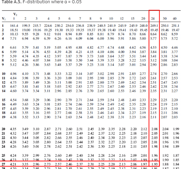
  • The critical value for the left tail is F(0.95,27,24). Since it is a left tail and we cannot find the 0.95 in the f- f-table, we must switch the degrees of freedom and then take a reciprocal of the final answer.
F-distribution table (Table A.5) at alpha=0.05, used to find the critical value after switching degrees of freedom for the left-tailed delivery-time example
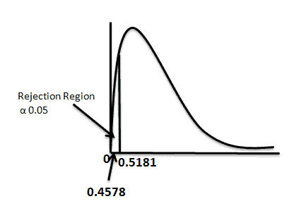
  • Reciprocal of F(0.05,24,27) = 1/F(0.025,24,27) = 1/1.93 = 0.5181
  • Calculate the F value F = S12/ S22
  • For left-tailed test keep the lowest variance as the numerator and the highest variance as the denominator = 38/83 = 0.4578
F-distribution curve for the left-tailed delivery-time example, with the rejection region (alpha=0.05) below the critical value 0.5181, and the calculated F-value 0.4578 falling inside the rejection region

Interpret the results:

Compare f calc to f critical. In hypothesis testing, a critical value is a point on the test distribution that is compared to the test statistic to determine whether to reject the null hypothesis. Since the f cal value is less than the f critical value, and it is in the rejection region. Hence, we reject the null hypothesis at a 95% confidence level.

F Test Left Tailed Excel Template

Unlock Additional Members-only Content!

To unlock additional content, please upgrade now to a full membership.
Upgrade to a Full Membership
If you are a member, you can log in here.

Helpful Videos

https://www.youtube.com/watch?v=FlIiYdHHpwU

When you’re ready, there are a few ways I can help:

First, join 12,000+ other Six Sigma professionals by subscribing to my email newsletter. A short read every Monday to start your work week off correctly. Always free.

* * *

If you’re looking to pass your Six Sigma Green Belt or Black Belt exams, I’d recommend starting with my affordable study guide:

1)→ 🟢Pass Your Six Sigma Green Belt: a study guide organized by the exam Body of Knowledge, 1,000+ practice questions with detailed answer explanations, and 8 full-length mock exams

2)→ ⚫Pass Your Six Sigma Black Belt: the full Black Belt Body of Knowledge, 2,000+ practice questions with detailed answer explanations, and 8 full-length mock exams

You’ve spent so much effort learning Lean Six Sigma. Why leave passing your certification exam up to chance? This comprehensive study guide offers 1,000+ exam-like questions for Green Belts (2,000+ for Black Belts) with full answer walkthroughs, access to instructors, detailed study material, and more.

​ Thousands have used this system to prepare. Join them here.