What is Non-Linear Regression?

Non-linear regression, aka Attributes Data Analysis, is organized into discrete data types (groups or categories).

When do you use Non-Linear Regression, aka Attributes Data Analysis?

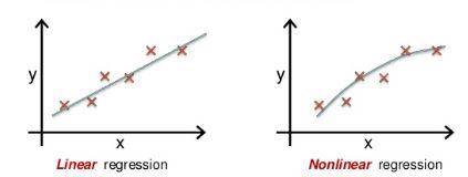
Simple Linear regression is a statistical technique used to estimate the mathematical relationship between a dependent variable (usually denoted as Y) and an independent variable (usually denoted as X) and is denoted with a straight line y=mx+b. Although statistical linear models could describe the classic straight line, most statistically linear models are not represented by straight lines but by curvilinear graphs. Non-linear regression, aka Attributes Data Analysis, is used to explain the nonlinear relationship between a response variable and one or more predictor variables (mostly curve line). In other words, a regression model is called “non-linear” if the derivative of the model depends on one or more parameters.

Specifically, use non-linear regression instead of ordinary least square regression when one cannot adequately model the relationship with linear parameters.

DO NOT USE Linear Regression for attribute data analysis- because this assumes the response variable is continuous.

For instance, Analyze attribute data using logit, probit, logistic regression, etc., to investigate sources of variation.

Logistic Regression

Logistic regression is a method used to predict a dependent variable for a given set of independent variables, such that the dependent variable is categorical. This method is widely used in machine learning algorithms.

Logistic regression is similar to linear regression; however, logistic regression predicts categorical data (like true or false), whereas linear regression predicts continuous data. Hence, the dependent variable in logistic regression is categorical, but in linear regression, the dependent variable is always continuous. Logistic regression uses a logit transformation on the dependent variable to fit a linear regression model.

The outcome of logistic regression is always categorical when the resultant outcome always has only two possible values of 0 or 1.  In logistic regression, the graph is not a linear line, but the line looks like a curve goes between 0 and 1. The curve is called the “S” curve and is also called as Sigmoid curve.

Although logistic regression tells the probability, it is most commonly used for classification. The team has to determine the threshold value if the probability of the event happening between 0 and 1, then based on the threshold value event is to be classified as 0 or 1.

For example, if the threshold value is 0.5, then any value between 0.5 and 1 it should be classified as 1, similarly any value below 0.5 then it should classify as 0

Logistic Regression calculation

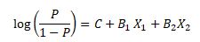
P ranges between 0 and 1; it represents the probability of an event to happen.

X₁ and X2 are the independent variables that determine the occurrence of an event.

C is the constant

B₁, B₂ represents the respective coefficients of X₁, X₂

Additional Notes on Logistic Regression

• The regression coefficients for logistic regression models are based on MAXIMUM LIKELIHOOD ESTIMATION.
• Sample sizes should be at least 50 per variable.
• Logistic Regression is best for:
  • Binary with two categories
  • Ordinal or Nominal w/ 3 or more categories

Logistic Regression Example

We can use Non-linear regression models in the analysis phase of DMAIC. For example, the American Cancer Institute wants to predict the chances of throat cancer based on the smoker’s average cigarette consumption per day. From the below random data, 0 indicates no cancer, and 1 indicates throat cancer.

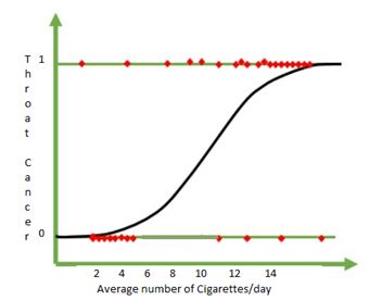
From the above data, logistic regression helps to assess what level of cigarette consumption leads to throat cancer. Moreover, from the above graph, one can say if the number of cigarette consumption is more than eight, it leads to throat cancer, and if cigarette consumption is below eight, there is no cancer. Hence, logistic regression is the best method for complex problems.

Certainly, we have to use statistical tools (like R and Minitab) to model the logistic regression.

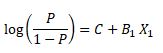
Using the formula

Suppose we get the following values (random values) from the above information

C= -0.100245

B1= 0.1814

If we want to predict 2.6

=-0.100245+ 0.1814*2.6= -0.53081

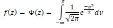
Use the sigmoid function to find the probability

Since the f(z ) value is 0.37 (towards zero), we can predict 2.6, there will be no chance of throat cancer.

Logit Analysis

Logit Analysis

Logit analysis is used when the response variable is categorical, especially when the outcome has two possible results, such as pass/fail, yes/no, alive/dead, or defect/no defect.

The key idea behind logit analysis is that we model the log odds of an event, rather than modeling the probability directly.

The standard logit formula is:

logit(p) = ln(p / (1 – p))

Where:

• p is the probability that the event occurs.
• 1 – p is the probability that the event does not occur.
• p / (1 – p) is the odds of the event occurring.
• ln means the natural logarithm, or log base e.

This is an important notation point. In many statistics texts and software outputs, the word log often refers to the natural logarithm. However, to avoid confusion, it is clearer to write the formula as ln(p / (1 – p)).

Why Use the Logit?

Probabilities are limited to values between 0 and 1. That creates a problem if we try to model probability directly with a straight-line equation because a linear model can produce values below 0 or above 1.

The logit transformation solves this by converting probabilities into log odds. Log odds can range from negative infinity to positive infinity, which makes them suitable for regression modeling.

Once the regression model is built, the logit value can be converted back into a probability using the logistic function:

p = 1 / (1 + e^-z)

Where:

• p is the predicted probability of the event.
• e is Euler’s number, approximately 2.718.
• z is the linear prediction from the regression equation.

Logit Regression Equation

A basic logit regression model has the following form:

z = β₀ + β₁x₁ + β₂x₂ + … + β_nx_n

Where:

• β₀ is the intercept.
• β₁, β₂, … β_n are the coefficients for the predictor variables.
• x₁, x₂, … x_n are the independent variables.

After calculating z, the logistic function converts that value into a probability between 0 and 1.

Logit Analysis Example

Suppose a cardiology doctor wants to predict the probability of a life-threatening outcome based on a patient’s cholesterol level. The response variable is binary: the patient is either alive or deceased.

The doctor may collect data showing cholesterol levels and the number of patients in each outcome group. From that data, the doctor can calculate the proportion of patients in the outcome category of interest.

The general steps are:

1. Calculate the proportion: p = event / total.
2. Calculate the odds: p / (1 – p).
3. Calculate the logit using the natural logarithm: ln(p / (1 – p)).
4. Use statistical software, such as Minitab, R, Python, or Excel, to estimate the regression equation.
5. Use the final model to predict the probability of the event at a given cholesterol level.

For example, if the probability of an event is 0.75, then:

Odds = 0.75 / (1 – 0.75) = 0.75 / 0.25 = 3

Logit(p) = ln(3) = 1.099

This means the log odds of the event are 1.099. A positive logit value means the event is more likely than not. A negative logit value means the event is less likely than not. A logit value of 0 means the event has a probability of 0.5.

Common Source of Confusion: log vs. ln

One common source of confusion is the word log. In some settings, especially in basic math or engineering contexts, log may mean log base 10. In logistic regression, however, the logit function uses the natural logarithm.

For clarity, the formula should be written as:

logit(p) = ln(p / (1 – p))

Using log base 10 would produce different numerical values. The standard logit values used in logistic regression are based on the natural logarithm.

Once the model is created, the predicted logit can be converted back into a probability. This allows the team to estimate the likelihood of a specific outcome and classify the result if needed.

Probit Analysis

The probit model was first introduced by Chester Bliss in 1934, but Ronald Fisher proposed the maximum likelihood method as an appendix to Bliss in 1935.

A probit model is a popular ordinal or binary response model specification. This model, which employs a probit link function, was estimated using the maximum likelihood method, hence this estimation was named probit regression.

z= β₀+ β₁x₁+ β₂x₂+………………+ β_nx_n

Where f is the standard normal cumulative distribution function (cdf)

Probit Analysis Example

A coaching center interested in students’ GMAT (Graduate Management Admission Test ) scores and admission into the business school. The response is a binary variable (i.e, admit or no admission into the business school)

Firstly, find the logarithm base 10 for the GMAT Score

Then, calculate the proportion of no admission = No admission /(admission + no admission)

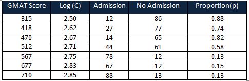
Lastly, calculate the Probit values using the chart

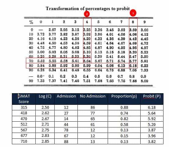
Calculate the slope and intercept using probit values and log values of the GMAT score.

We must use statistical tools (like R and Minitab) to model the logistic regression.

Once the model was established, the probit function was to find whether the chances of student admission or no admission into the business school for a particular GMAT score.

Difference between logit and probit

Both logit and probit models yield almost the same results. The logit and probit functions are increasing, and both functions increase relatively quickly in the central portion and relatively slow at the extremities, and both functions lie between 0 and 1. While the only key difference between the logit and probit models is in the use of the link function

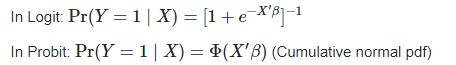
In other words, the logit model will have slightly flatter tails compared to the probit model. 

When you’re ready, there are a few ways I can help:

First, join 30,000+ other Six Sigma professionals by subscribing to my email newsletter. A short read every Monday to start your work week off correctly. Always free.

—

If you’re looking to pass your Six Sigma Green Belt or Black Belt exams, I’d recommend starting with my affordable study guide:

1)→ 🟢Pass Your Six Sigma Green Belt​​

2)→ ⚫Pass Your Six Sigma Black Belt ​​​

You’ve spent so much effort learning Lean Six Sigma. Why leave passing your certification exam up to chance? This comprehensive study guide offers 1,000+ exam-like questions for Green Belts (2,000+ for Black Belts) with full answer walkthroughs, access to instructors, detailed study material, and more.

​ Join 10,000+ students here.