
Central Tendency

What is Central Tendency?

Central tendency refers to the statistical measure used to determine the center of a distribution of a data set. We also call it a measure of central location. In other words, the single value most represents the entire data set.

Central tendency reflects the principle that when using normal data, all three of the main measures (mean, mode, median) tend to be roughly the same.

When Do You Use It?

Central Tendency is the widely used method in basic data analysis. Based on the situation, the central tendency measure could be Mean, Median, or Mode.

Mean (Average)

The mean is a well-known measure of central tendency, and it is also the most commonly used method for measuring the center value of a continuous data set. The mean is the total of all data values divided by the number of data points, and it is also called the arithmetic mean. Different types of means exist: like the arithmetic mean, geometric mean, weighted mean, etc. The notation for the population mean is represented with μ (“Mu”), whereas the sample mean is represented as X̅.

Central Tendency

Where X represents each number and n is the sample size.

One advantage of the mean: you are not required to sort the data. Likewise, it uses all the data values for the calculations.

The disadvantage of the mean is that the data is influenced by outliers, and the mean is not the actual value of any data point.

Median

The median is the middle value when the data is arranged in ascending or descending order. If the data set has even values, then the median is the average of the middle two values.

An advantage of the median is it provides an idea of where most of the data is located, and also, it is not impacted by outliers.

A disadvantage is that the data must be sorted and arranged, and the median has more variation than mean

Mode

The mode is the value that occurs most often in the data set. It is possible for groups of data to have more than one mode if multiple numbers are tied for the greatest frequency in the data set. In the histogram, we can identify the mode with the highest bar.

An advantage of Mode is that there is no need to sort the data, unlike the median, and it is not influenced by outliers.

A disadvantage of Mode is sometimes it will have multiple modes, and a few times, no mode in the data set.
Central Tendency

Notes about Central Tendency

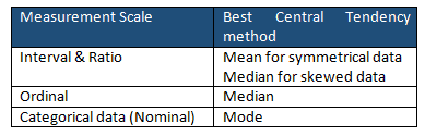
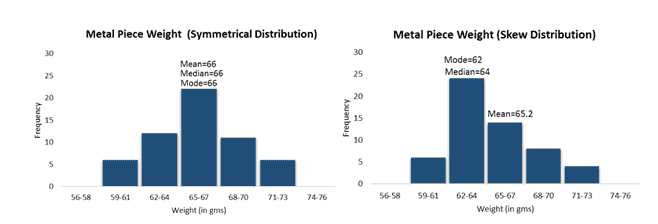
The most common assumption of a statistical test is that data is normally distributed. For normally distributed data, we can use any of the central tendency methods (mean, mode, or median) because, for symmetrical data, all three values are equal. However, most statisticians use the mean as it considers all the values in the data set for calculation, and if any value changes, it will affect the mean.

The median is the best central tendency method: as the skew increases, the difference between the mean and median will also increase.
Central Tendency
Example: Comparison between Symmetrical and Skewed Distribution

A central tendency is rarely perfectly centered. Even if it was, it wouldn’t stay that way. As time goes on, a standard deviation can drift over 1.5 sigmas over time.

Without a 1.5 sigma drift, a 6 Sigma process would only generate 2 defects per BILLION! As it is, because of this drift, the errors are 3.4 per million.

Examples in DMAIC

Central Tendency is the widely used method in the Measure phase of DMAIC.

Example 1

Find the mean, median, and mode of weight distribution for a piece of metal.

Mean: What is the mean (average) weight of a metal piece (in gms)

56,55,52,55,51,48,58,59,63,50

Where N=10

Central Tendency

Median: What is the median weight of a metal piece (in gms)?

56,55,52,55,51,48,58,59,63,50

Sort the data

48,50,51,52,55,55,56,58,59,63

Since N=10 (even number), average the two middle values = 55+55/2 = 55

Mode: What is the mode of the distribution of a metal piece (in gms)?

56,55,52,55,51,48,58,59,63,50
Central Tendency

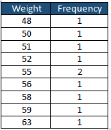
Since the frequency of the 55 weight is 2, therefor Mode of the weight distribution is 55.

Example 2

Find the cumulative frequency distributions using Central Tendency.

Mean, Median, and Mode of grouped data:
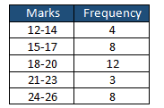
Central Tendency

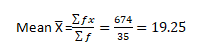
Since we don’t have exact marks for each individual, approximate Mean and Median values can be calculated using frequency distribution.

Find the mid marks of each class:
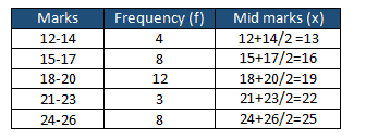
Multiply frequency with Mid marks:
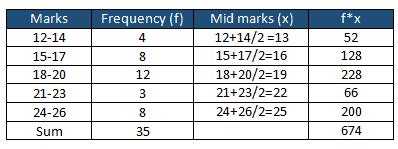
Central Tendency

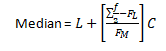
Median

  • Where L is the lower boundary of median class
  • FL = Cumulative frequency of lower class next to the median class
  • FM = Frequency of median class
  • C = Class width

Find the cumulative frequency:
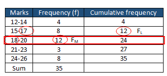
The sum of frequency Σf is 35, so Σf/2 =17.5

The smallest cumulative frequency greater than or equal to 17.5 is 24, and the corresponding median class is 18-20

The frequency of the median class is 12 (FM) and the Cumulative frequency of the lower class next to the median class is 12 (FL). When the data values are whole numbers, subtract 0.5 from the lower limit(18-0.5 =17.5) or add the first number from FM row (18) and the last number from the previous row (17) and divide by two. i.e (18+17)/2 =17.5

  • L= =17.5
  • FL =12
  • FM =12
  • C=14-12=3

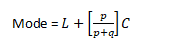
Mode

  • p= highest frequency minus the frequency of the next lower class
  • q= highest frequency minus the frequency of the next higher class
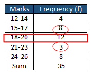
  • p=12-8=4
  • q=12-3=9

Videos on Central Tendency

Standard Deviation

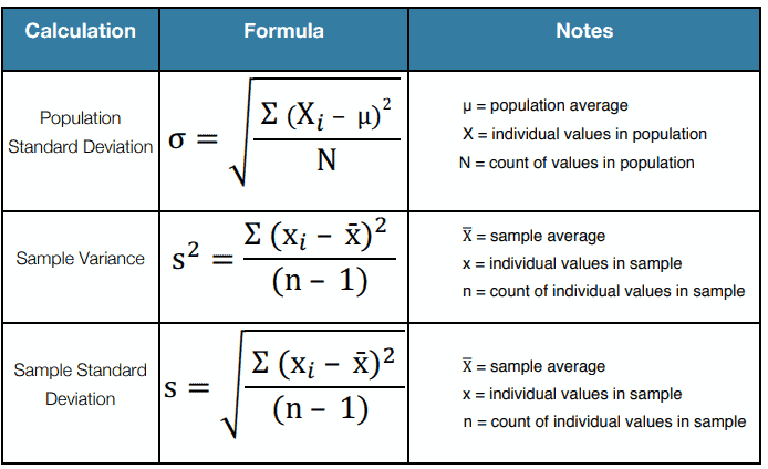
Standard deviation is used to measure the amount of variation in a process. This is one of the most common measures of variability in a data set or population.

There are 2 types of equations: Sample and Population.

What is the difference between Population and Sample?

Population refers to ALL of a set, and the sample is a subset. We most often have a sample and are trying to infer something about the whole group. However, if we want to know a truth of a subset of a whole population, use the Population equation.

Use Population When:

  1. You have the entire population.
  2. You have a larger population sample, but you are only interested in this sample and do not wish to generalize your findings to the population.

Use Sample When (Most often):

  1. If all you have is a sample but wish to make a statement about the population standard deviation from which the sample is drawn, you need to use the sample SD.

Remember: It is impossible to have a negative standard deviation.

How to Measure the Standard Deviation for a Sample (s)

Standard Deviation for a Sample (s)

  1. Calculate the mean of the data set (x-bar)
  2. Subtract the mean from each value in the data set
  3. Square the differences found in step 2.
  4. Add up the squared differences found in step 3.
  5. Divide the total from step 4 by (n – 1) for sample data
  6. (Note: At this point, you have the variance of the data).
  7. Take the square root of the result from step 5 to get the SD

Example of Standard Deviation for a Sample (s)

The length of 8 bars in centimeters is 9, 12, 13, 11, 12, 8, 10, and 11. Calculate the sample standard deviation of the length of the bar.

  1. Calculate the mean of the data set

(9+12+13+11+12+8+10+11)/8=86/8=10.75

2. Subtract the mean from each value in the data set

  • 10.75-9=1.75
  • 10.75-12=-1.25
  • 10.75-13=-2.25
  • 10.75-11=-0.25
  • 10.75-12=-1.25
  • 10.75-8=2.75
  • 10.75-10=0.75
  • 10.75-11=-0.25

3. Square the differences found in step 2.

  • (1.75)2 =3.06
  • (-1.25)2 =1.56
  • (-2.25)2 =5.06
  • (-0.25)2 =0.06
  • (-1.25)2 =1.56
  • (2.75)2 =7.56
  • (0.75)2 =0.56
  • (-0.25)2 =0.06

4. Add up the squared differences found in step 3 =19.50

5. Divide the total from step 4 by (n – 1) for sample data=19.5/8-1=2.79, so the variance is 2.79

6. Take the square root of the result from step 5, SD of sample bar length = 1.67

How to Measure the Standard Deviation for a Population (σ)

Standard Deviation for a Population (σ)

  1. Calculate the mean of the data set (μ)
  2. Subtract the mean from each value in the data set
  3. Square the differences found in step 2.
  4. Add up the squared differences found in step 3.
  5. Divide the total from step 4 by N (for population data).
    1. (Note: At this point, you have the variance of the data).
  6. Take the square root of the result from step 5 to get the SD

 Example of Standard Deviation for a Population (σ)

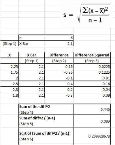
Nana’s Bakery wants to optimize the consistency of its cakes. The recipe calls for a certain number of eggs. The problem is that there is variation in egg sizes. Six eggs were randomly selected, and the following weights were recorded (measured in ounces).

2.25; 1.75; 2.0; 2.5; 2.3; 1.8

What is the SD of the egg weights?

standard deviation example

Standard Deviation and Variance

Variance is Std Dev ^2.

Std Dev = Sqrt(variance)

The Uniform Distribution

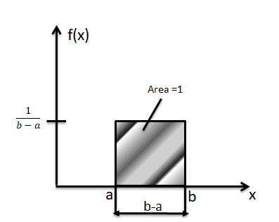
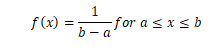
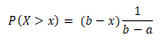
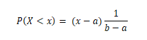
A uniform distribution is a continuous probability distribution. It describes the condition where all possible outcomes of a random experiment are equally likely to occur.  For the uniform distribution, the probability density function f(x) is constant over the possible values of x.

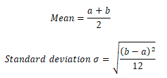
The formula for Mean and standard deviation of uniform distribution
Standard Deviation
Probability density function
The Area between p and q
Standard Deviation
Area right of x
Area left of x
Standard Deviation

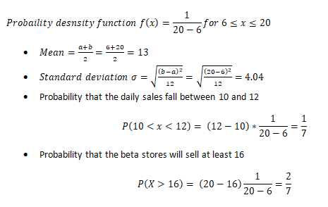
Example: The number of mobile phones sold by Beta stores is uniformly distributed between 6 and 20 per day. Then find

  • Mean
  • Standard deviation
  • Probability that the daily sales fall between 10 and 12
  • Probability that the Beta stores will sell at least 16

Let X be the number of mobiles sold daily by beta stores: X follows the uniform distribution over (6, 20). Thus the probability density function is:


Standard Deviation of Sample Proportion – Quality Control Example

Walkthrough: Standard Deviation of a Sample Proportion

Question: In a factory, 5% of manufactured bolts are known to be defective. A quality inspector randomly samples 400 bolts. What is the standard deviation of the sample proportion of defective bolts, assuming the distribution is approximately normal?

Step 1: Identify the known values

  • Population proportion (p) = 0.05
  • Sample size (n) = 400

Step 2: Use the standard deviation formula for a sample proportion

σp̂ = √[ p(1 − p) / n ]

Step 3: Plug in the values

σp̂ = √[ 0.05 × (1 − 0.05) / 400 ]
= √[ 0.05 × 0.95 / 400 ]
= √[ 0.0475 / 400 ]
= √0.00011875

Step 4: Calculate

√0.00011875 ≈ 0.0109

Final Answer:

The standard deviation of the sample proportion of defective bolts is approximately 0.0109.

Helpful Videos

Video on Variance

The Normal Curve

The Uniform Distribution

When you’re ready, there are a few ways I can help:

First, join 12,000+ other Six Sigma professionals by subscribing to my email newsletter. A short read every Monday to start your work week off correctly. Always free.

* * *

If you’re looking to pass your Six Sigma Green Belt or Black Belt exams, I’d recommend starting with my affordable study guide:

1)→ 🟢Pass Your Six Sigma Green Belt: a study guide organized by the exam Body of Knowledge, 1,000+ practice questions with detailed answer explanations, and 8 full-length mock exams

2)→ ⚫Pass Your Six Sigma Black Belt: the full Black Belt Body of Knowledge, 2,000+ practice questions with detailed answer explanations, and 8 full-length mock exams

You’ve spent so much effort learning Lean Six Sigma. Why leave passing your certification exam up to chance? This comprehensive study guide offers 1,000+ exam-like questions for Green Belts (2,000+ for Black Belts) with full answer walkthroughs, access to instructors, detailed study material, and more.

​ Thousands have used this system to prepare. Join them here. 

Stem and Leaf Plots

A stem-and-leaf plot (or stemplot) organizes numerical data, whether continuous or discrete, by splitting each value into a “stem” (all but the last digit) and a “leaf” (the final digit). It’s a compact way to sort, visualize distribution, and preserve the original data.

Stem and leaf offer a quick and novel way for simultaneously sorting and displaying data sets where each number in the data set is divided into two parts: a stem (all numbers except the last digit) and a leaf (only the last digit). For example, in the numbers 38 and 52, the stems are 3 and 5, while the leaves are 8 and 2.

Significance of Stem and Leaf Plot

Stemplots originated in early 1900s (Arthur Bowley) and were popularized by John Tukey in his 1977 Exploratory Data Analysis. They resemble histograms but retain actual data values, which is useful for visualizing distribution with precision.

Stem and leaf plots are some of the best ways to not only study but track information as well. Stem and leaf plots have been around for decades and are like a cross between a histogram and a check sheet. The difference with this type of graph is that it preserves the actual data as well as being the most like a frequency distribution.

Stem and leaf plots are methods for showing the frequency with which certain classes of values occur. It will organize data visually and will be able to interpret data and draw conclusions using the plot.

Uses

  • Effective for organizing and visualizing numeric data.
  • Supports quick calculation of median, mode, quartiles.
  • Enables direct comparison of multiple datasets with back-to‑back plots.
  • Retains original data values, unlike histograms.

How to Create a Stem-and-leaf plot

There are many different ways to create a stem and leaf plot but they all serve the same purpose at the end of the day.

  • Sort the data in ascending order.
  • Define stems and leaves (stem = all but last digit, leaf = last digit).
  • Draw a vertical line and list each unique stem in a left-hand column.
  • Map leaves to their stem, sorted ascending.
  • Add a key, e.g., “2 | 7 = 27.”
  • Compute descriptive stats (median, quartiles, mode) directly from the stemplot.                                       

Example

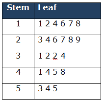
Example: A teacher asked 23 of her male students how many books they had read in the last 4 years. Draw a stem and left diagram for the following data.

32,55,12,18,23,26,24,28,44,53,27,16,14,34,29,31,41,17,11,32,54,48,45

First, Sort the numerical values in ascending order

11,12,14,16,17,18,23,24,26,27,28,29,31,32,32,34,41,44,45,48,53,54,55

Analyze the data and determine stem and a leaf: The minimum value is 11 and the maximum value is 55.

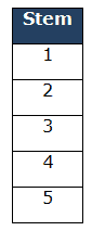
Draw a line and lists the possible stems in a single column from lowest to highest on the left side of the line.

Then for each stem, record all the leaves associated with that stem. Also, note that leaves are in numerical order.

Key: 2|7 means 27 books

Total count values =23

  • Median:
    • median = (n+1)/2-th value: (23+1)/2 = 12th value in the list
  • Mode: The number which appears most often in a set of numbers= 32 number repeated twice. Hence Mode is 32 books.
  • Q1 (Lower Quartile) = Find ¼ (n+1) =24/4=6th value is 18 books.
  • Q3 (Upper Quartile) = Find ¾(n+1)= 3*24/4= 18th value is 44 books.
  • The Quartile range = 44-18 = 26 books.

Back to Back stem-and-leaf-plot

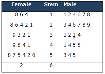
Back to back stem and leaf diagrams can be used to compare different sets of data relating to the same subject. In other words, it helps to compare different sets of data together at the same time.

Example: For the above example, add 23 female students’ books reading data.

Sort the data in ascending order for both male and female. Then identify the stem and respective leaves for male and female.

Stem and Leaf Plots

Stem-and-leaf-plot with Decimals

There are some stem and leaf plots out there that have decimals along with it. When you are tracking your leaves, all you have to do is include the decimal points as well.

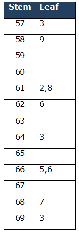
It is not that different from a normal stem and leaf plot, only in which you have to designate your stems and leaves to where you want them to begin. For instance, your stems may be the ones place while your leaves are the decimal points. It is all in how you do the graph and what numerical information you are trying to convey. Stem and leaf plots are very flexible this way.

Example: The average heights of ten high school students in inches are reported below. Draw a stem and left diagram for the following students’ heights data.

61.2, 69.3, 58.9, 57.3, 61.8, 62.6, 66.5, 68.7, 66.6, 64.3

Stem and Leaf Plots

Stem and Leaf Plot Activities

There are many different activities in which you can involve a stem and leaf plot. For example, If there is a football game going on, you can track the number of yards someone has run; to make stem and leaf plots even more fun, you can even track the score in a video game and see who has the highest data on the plot.

There is no shortage of activities, usefulness, and fun a stem and leaf plot can achieve. It is up to you to find out the different ways to utilize them and make your own graph.

Videos

Notes on Stem and Leaf Plots

  • Box Plots, Histograms, and Stem and Leaf plots all display the same data.
  • Histograms are better when you only care about shape and have large datasets. Stemplots preserve data values and work best with medium-sized datasets.

When you’re ready, there are a few ways I can help:

First, join 12,000+ other Six Sigma professionals by subscribing to my email newsletter. A short read every Monday to start your work week off correctly. Always free.

* * *

If you’re looking to pass your Six Sigma Green Belt or Black Belt exams, I’d recommend starting with my affordable study guide:

1)→ 🟢Pass Your Six Sigma Green Belt: a study guide organized by the exam Body of Knowledge, 1,000+ practice questions with detailed answer explanations, and 8 full-length mock exams

2)→ ⚫Pass Your Six Sigma Black Belt: the full Black Belt Body of Knowledge, 2,000+ practice questions with detailed answer explanations, and 8 full-length mock exams

You’ve spent so much effort learning Lean Six Sigma. Why leave passing your certification exam up to chance? This comprehensive study guide offers 1,000+ exam-like questions for Green Belts (2,000+ for Black Belts) with full answer walkthroughs, access to instructors, detailed study material, and more.

​ Thousands have used this system to prepare. Join them here. 

6M’s in Six Sigma (Six Ms or 5Ms and one P or 5M1P)

In the Analyze phase of DMAIC, we want to identify the root cause of the defects that are causing variation in our process. Sometimes the culprits are easy to identify. We use the 6M’s in Six Sigma (Six Ms or 5Ms and one P or 5M1P) to find the possible root cause of the process variation or problems. More often, we have to hypothesize what is causing the variation and then test that hypothesis to see if our hunch was right. But how do you come up with a hypothesis for what is causing variation?

In Six Sigma, we describe process variation in terms of 6M’s (aka 5 M’s and 1 P). These are six elements that contribute to variation in a process. Those six elements – 5 Ms and on P (or 6Ms) influence variation in all processes – manufacturing or not.

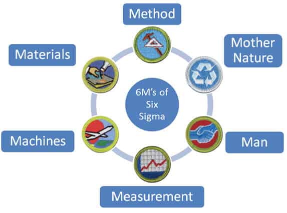
The 5Ms and one P is a concept that is a quality management and problem-solving methodology, particularly in the manufacturing industry. They represent six potential sources of problems or causes for variations in a process. The 5Ms stand for:

6M's in Six Sigma
6M’s of Six Sigma

Ishikawa states the 6 Ms (also known as the 5 Ms and 1 P) as Man, Machine, Material, Method, Measurement, and Mother Nature.

  1. Method
  2. Mother Nature’s “Environmental”
  3. (Man) People
  4. Measurement
  5. Machine
  6. Materials

Let’s Takes A Look at 6M’s in Six Sigma (Six Ms or 5Ms and one P or 5M1P) Attributes

6 Ms in Manufacturing Example

  1. Method: Method refers to the procedures, instructions, and techniques used to carry out the process. It includes standard operating procedures (SOPs), work instructions, process flow, and overall process design.
    • Following an assembly line is much different than a manufacturing floor that does not.
  2. (Man) People: Man refers to the human resources involved in the process, including operators, technicians, and supervisors. It focuses on the skills, training, and expertise of the people performing the tasks.
    • Empowering any single employee to stop the entire production line if he finds a defect.
  3. Measurement: Involves the measurement systems and instruments used to assess and monitor the process. It focuses on the accuracy, precision, calibration, and reliability of measurement devices.
    • If the supplier measures in English units and the manufacturer measures in metrics, issues could arise.
  4. Machine: Machine represents the equipment, machinery, and tools used in the process. It includes factors such as machine capability, maintenance, calibration, and reliability.
    • The age and robustness of the machine may impact the process.
  5. Materials: Encompasses the raw materials, components, and supplies used in the process. It involves aspects like material quality, specifications, storage conditions, and handling procedures.
    • Some materials are harder to work with than others.
  6. Mother Nature’s “Environmental”: This additional factor is sometimes included to represent the physical surroundings or conditions in which the process takes place. It includes factors like temperature, humidity, lighting, cleanliness etc
    • Ambient humidity may cause more breakdowns in machines than normal.

6 Ms in Management

  1. Method
    • If one team is developing software following a Waterfall approach while a second is using an Agile practice and a third is using Kanban, each method is different.
  2. Mother Nature’s “Environmental”
    • Offices in the north are more lenient to snow days than those in the south.
  3. (Man) People
    • People untrained in 6 Sigma tend to focus on the ‘Man’ portion of the 6Ms when looking at a process.
    • A manager who is unenlightened in six sigma is most likely going to focus on Man. Unenlightened managers tend to think of the process performance as being influenced more by the person component than by the other five components of the six Ms of the machine, material, method, measurement, or mother nature. (Don’t ask whom, ask why.)
  4. Measurement
    • It’s difficult to evaluate teams evenly if each team leader rewards their teams for different behaviors.
  5. Machine
    • Software development productivity may be different if developers have slower machines or worse tools to use.
  6. Materials
    • Employees can only build a product as good as the raw materials they get.

How to develop a Cause and Effect Diagram using 5Ms and 1P

The Cause and effect diagram is a structured graphical diagram listing all possible causes and their relationship with the main effect or problem. The diagram’s basic input is the brainstorming that pushes to identify all the possible causes rather than just more noticeable ones.

Following are the steps to draw a fishbone diagram:

1: Identify the problem:

  • Identify and clearly write down the effect or a problem that needs to be analyzed
  • Then create an operational definition of a problem to ensure all the stakeholders will understand it
6M's in Six Sigma

2: Determine Effect or Problem:

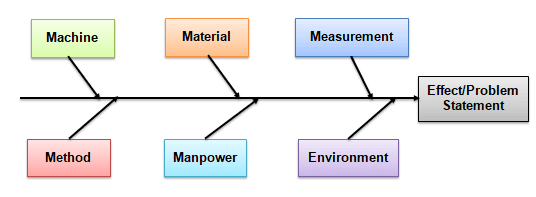
  • Draw a horizontal line. This is a spine
  • At the end of the spine, towards the right, draw a box and determine the description of an effect 
6M's in Six Sigma

3: Identify major causes contributing to the effect or a problem

  • Establish main causes and write down a few main causes above the horizontal line and a few below the horizontal line. Make sure they are placed on the tail of the same arrows.
  • Each cause or reason for imperfection is a source of variation. Causes are usually grouped into major categories to identify these sources of variation.
  • Man/People: Anyone involved with the process.
  • Methods: How the process is performed and the specific requirements for doing it, such as policies, procedures, rules, regulations, and laws.
  • Machines: Any equipment, computers, tools, etc., required to accomplish the job.
  • Materials: Raw materials, parts, pens, paper, etc., used to produce the final product.
  • Measurements: Data generated from the process that is used to evaluate its quality.
  • Environment: The conditions, such as location, time, temperature, and culture, in which the process operates.
6M's in Six Sigma

4: Identify sub causes

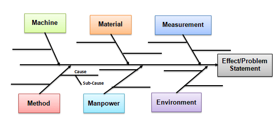
  • Identify as many sub-causes that are relevant to the main causes
  • For instance, if the sub-cause applies in multiple places, list it under each main category.
6M's in Six Sigma

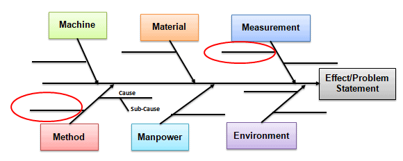
5: Analyze the diagram

  • At this time, the fishbone diagram shows all the possible causes of an effect.
  • Identify causes that are not impacting the effect and also identify causes that need further investigation.
  • Further, perform a 5Why analysis of the identified causes (also called noises) to arrive actual root cause.
6M's in Six Sigma (Six Ms or 5Ms and one P or 5M1P)

Six Sigma 5M and 1P Example

By and large, Fishbone diagrams are used to identify the root causes of a problem in the “Analyze” phase of Six Sigma’s DMAIC (Define, Measure, Analyze, Improve, and Control).
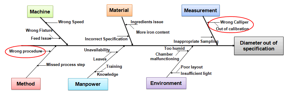
Example: XYZ is a valve manufacturing unit receiving persistent customer complaints about the valve diameter. The plant’s General Manager asked QA and Production team to conduct a root cause analysis. So, the team performed Brainstorming and drew the Cause and Effect diagram to identify all the possible causes.

6M's in Six Sigma (Six Ms or 5Ms and one P or 5M1P)

The team identified that the wrong caliper and wrong procedures were the probable causes. Further, the team has to perform a 5 Why analysis to identify the root cause.

6M’s in Six Sigma (Six Ms or 5Ms and one P or 5M1P) Template Download

Benefits of 6M’s in Six Sigma (Six Ms or 5Ms and one P or 5M1P)

  • The framework helps in troubleshooting, root cause analysis, and implementing effective corrective actions to improve quality, productivity, and overall performance.
  • Further, it graphically displays all the possible causes related to a problem to discover the root causes.
  • Helps the team to focus on the problem and brainstorm until the elimination of the root cause.
  • Easy to implement in any case.

6M Insights

  • When you have a bell-shaped curve, none of the 5 Ms or one P are unduly influencing the process.
  • Six elements contribute to variation in a process. Those six elements – 5 Ms and on P (or 6Ms) influence variation in all processes – manufacturing or not.
  • You could also use the 6M approach as a spine on each of the fishbone diagrams and then ask the 5 whys to narrow down the potential root cause.

5 m’s and one p

6M’s in Six Sigma (Six Ms or 5Ms and one P or 5M1P) Practice Questions

Unlock Additional Members-only Content!

To unlock additional content, please upgrade now to a full membership.
Upgrade to a Full Membership
If you are a member, you can log in here.

Thank You for being a Member!

Here’s some of the bonus content that is only available to you as a paying member.