Linear regression is a statistical technique used to estimate the mathematical relationship between a dependent variable (usually denoted as Y) and an independent variable (usually denoted as X). In other words, predict the change in the dependent variable according to the change in the independent variable.
- Dependent variable or Criterion variable – That is the variable for which we wish to make a prediction.
- Independent variable or Predictor variable – The variable used to explain the dependent variable.
When to Use Linear Regression
In simple linear regression, there is only one independent variable that is used to predict a single dependent variable. Whereas in multiple linear regression, we use more than one independent variable to predict a single dependent variable. In fact, the basic difference between simple and multiple regression is in the presence of explanatory variables.
For example, compare the crop yield rate against the rainfall rate in a season.
Notes about Linear Regression
The first step of linear regression is to test the linearity assumption. This can be performed by plotting the values in a graph known as a scatter plot to observe the relationship between the dependent and independent variables. If the data is exponentially scattered, then there is no point in creating the regression equation.
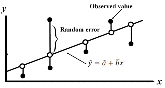
Draw the line which covers the majority of the points; furthermore, we can consider this line as the “best fit” line
The mathematical equation of the line is y=a+bx+ε.
Where:
- b – Slope of the line
- a – y-intercept when x=0
- Random error (ε-Epsilon) – The difference between an observed value of y and the mean value of y for a given value of x.
Assumption of Linear regression
- Linear relationship between the dependent and independent variable.
- All variables of regression to be multivariate normal.
- Particularly there is no or little multicollinearity in the data.
- Response variable is continuous, and also residuals are almost the same throughout the regression line.
The method of Least Squares
The method of least squares is a standard approach in regression analysis to determine the best-fit line for a given data. It basically provides a visual relationship between the given data points.
In general, the dependent variables are demonstrated on the y-axis, while the independent variables are demonstrated on the x-axis. The least square method determines the position of a straight line, which we also call a trend line or the equation of the line. This straight line is also known as the best-fit line.
The least square method means that the overall solution minimizes the sum of squares of the errors made in the results of every single equation. For instance, we can use them to find the values of the coefficients a and b.


We can compute the least-square estimator of a and b as follows:
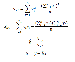
Compute â and b̂ values and then substitute these values into the equation of a line to obtain the least squares prediction equation or regression line.
Linear Regression example in DMAIC
Example: Linear Regression is specifically used in Analyze phase of DMAIC to estimate the mathematical relationship between a dependent variable and an independent variable.
A passenger vehicle manufacturer is reviewing the 10 salespersons’ training records. In fact, their main aim is to compare the salesperson’s achieved target (in %) with the number of sales module trainings completed.
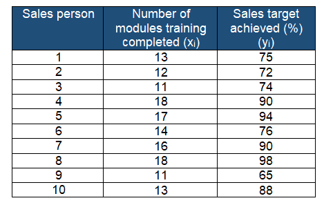
Compute the least square prediction equation or regression line.

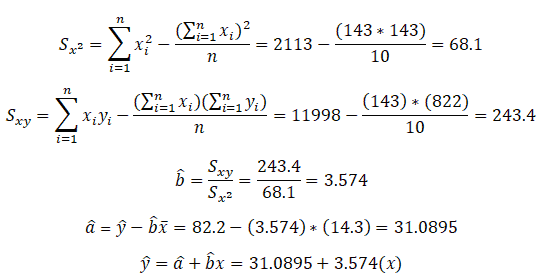
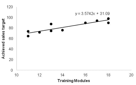
Furthermore, predict y for a given value of x by substitution into the prediction equation. For example, If a salesperson completes 15 training modules, then the predicted achieved target sales would be:
ŷ = 31.09+3.5742(15)= 84.7019=84.7%
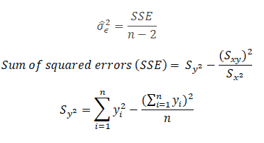
Estimate the variability of random errors
Referring the mathematical equation of the line is y=a+bx+ε, and also the least square line is:

A random error (Є) affects the error of prediction. Hence, the variability of the random errors (σε2) is the key parameter while predicting by the least squares line.
Estimate variability of the random error σε2
Example: From the above data, compute the variability of the random errors:
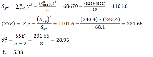
From the above calculation, σ̂Є is 5.38. Thus, most of the points will fall within ±1.96 σ̂Є i.e 10.54 of the line. Hence, approx 95% of the values should be in this region. Moreover, from the above graph, it is clearly evident that all the values are within ±10.54 of the line.
Test of the slope coefficient
If we set b equal to 0, then we can test whether or not the existence of a significant relationship between the dependent and independent variables. If b is not equal to 0 there is a linear relationship. The null and alternative hypotheses are:
- The null hypothesis H0: b=0
- The alternative hypothesis H1: b≠0
Degrees of freedom = n-2

Example: From the above data determine if the slope results are significant at a 95% confidence level.
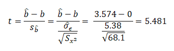
Determine the critical values of t for 8 degrees of freedom at a 95% confidence level.
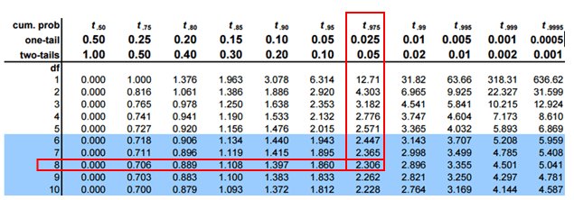
t0.025, 8 = -2.306 and 2.306
The calculated t-value is 5.481, which is not in between -2.306 and 2.306. We can reject the null hypothesis if the t-value is greater than 2.306 or less than -2.306.
In this case, we can reject the null hypothesis and conclude that b≠0 and there is a linear relationship between the dependent and independent variables.
Confidence interval estimate for the slop b
The confidence interval estimate for the slope b is:
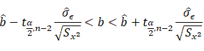
Example: from the above data, compute the confidence interval around the slope of the line:

2.0707<b<5.07
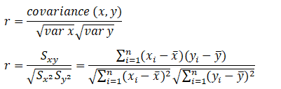
Correlation Coefficient
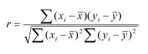
The linear correlation coefficient r measures the strength of the linear relationship between a sample’s paired x and y values.
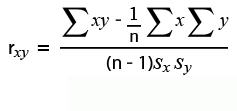
Pearson’s Correlation Coefficient
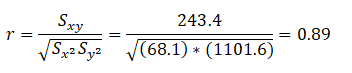
Example: From the above data, find the correlation coefficient:
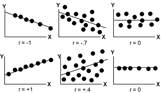
Note that -1≤ r ≤ +1:
- The line slopes upward to the right when r indicates a positive value.
- The line slopes downward and to the right when r indicates a negative value.
- A value closer to 1, indicates the stronger positive linear relationship.
- A value closer to -1, indicates the stronger negative linear relationship.
- When r=0 implies no linear correlation.
How is correlation analysis used to compare bivariate data?
The Measure of central tendency, variance, or spread, summarizes a single variable. It does this by providing important information about its distribution as can be seen below in the example. Often, more than one variable is collected in a study or experiment. The resulting data are bivariate when two variables are measured on a single experiment unit. For example, job satisfaction is stratified by income.
In most instances, in bivariate data, it determines that one variable influences the other variable. Furthermore, the quantities from these two variables are often represented using scatter plots to explore the relation between the two variables.
Bivariate data can be described with graphs and numerical measures depending on the data type. If one or both variables are qualitative, use a pie chart or bar chart to see the relationship between variables. For example, compare the relationship between opinion and gender. If the two variables are quantitative, use the scatter plot. The Correlation Coefficient is often used in comparing bivariate data.
Example:
Correlation between the amount of time spent in a Casino (independent variable) and the amount ($) lost (dependent variable).
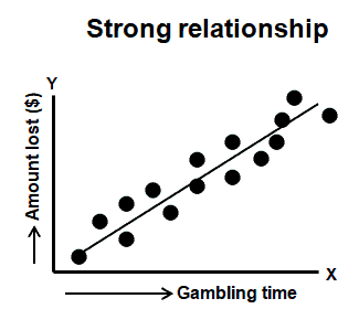
The correlation coefficient varies between -1 and +1. Values approaching -1 or +1 indicate a strong correlation (negative or positive), and values close to 0 indicate little or no correlation between x and y.
Correlation does not mean causation.
A positive correlation can be either good news or bad news.
A negative correlation is not necessarily bad news. Moreover, it merely means that as the independent variable goes more negative, the dependent variable also goes negative.
r = 0; does not indicate the absence of a relationship, a curvilinear pattern may exist; r=-0.76 has the same predictive power as r = +0.76.
Correlation Coefficient Videos
Coefficient of determination (R2)
The coefficient of determination is the proportion of the explained variation divided by the total variation when linear regression is performed.
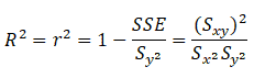
r2 lines in the interval of 0≤ r2 ≤1.
Example: Now that we have the above data, compute the coefficient of determination.

We can say that 79% of the variation in the overall number of training modules completed explains the variation in the sales targets.
Linear Regression-Related Topics
Residual Analysis: “Because a linear regression model is not always appropriate for the data, you should assess the appropriateness of the model by defining residuals and examining residual plots.”
Linear Regression Additional Videos
When you’re ready, there are a few ways I can help:
First, join 30,000+ other Six Sigma professionals by subscribing to my email newsletter. A short read every Monday to start your work week off correctly. Always free.
—
If you’re looking to pass your Six Sigma Green Belt or Black Belt exams, I’d recommend starting with my affordable study guide:
1)→ 🟢Pass Your Six Sigma Green Belt
2)→ ⚫Pass Your Six Sigma Black Belt
You’ve spent so much effort learning Lean Six Sigma. Why leave passing your certification exam up to chance? This comprehensive study guide offers 1,000+ exam-like questions for Green Belts (2,000+ for Black Belts) with full answer walkthroughs, access to instructors, detailed study material, and more.

Comments (11)
link does not work
Ted the link doesn’t work.Could you kindly provide a valide one?Thank you!
Hi all, Updated with a few links and a few videos. Let me know how this works for you!
Best, Ted.
All your contributions are very useful for professionals and non-professionals. I appreciate your availability to share these types of great and valuable info And you did it very well! Can’t wait to read more… You nailed it……..
Thanks for the kind words, Lyla!
Ted,Can you explain how the 1.96 and10.54 is derived?
From the above calculation σ̂Є is 5.38. Thus, most of the points will fall within ±1.96 σ̂Є i.e 10.54 of the line, hence approx 95% of the values should be in this region. Moreover from the above graph, it is clearly evident that all the values are within ±10.54 of the line.
Anshika,
A random error (Є) affects the error of prediction. Hence the variability of the random errors (σε2) is the key parameter while predicting by the least squares line.
Random errors in experimental measurements are caused by unknown and unpredictable changes in the experiment. Random errors often have a Gaussian normal distribution.
For the standard normal distribution, P(-1.96 < Z < 1.96) = 0.95, i.e., there is a 95% probability that a standard normal variable, Z, will fall between -1.96 and 1.96. (refer Z table)
From the calculation variability of random error is 5.38. 1.96 *5.38 = 10.54. 95% of values should be in this region, but If you observe above graph (in the example) all the points fall with in ± 10.54 of the LS line.
Hope this clarifies!
Thanks
I appreciate how this blog not only covers the basics of linear regression but also delves into advanced topics. It’s a comprehensive resource that grows with you as you advance in your understanding
Thanks for the kind note, Zara. We’ve put a lot of effort in and it’s gratifying to see that it helps people!
The link for the correlation coefficient leads to this same page.
Hi Lillian,
Yes, sometimes I combine concepts together on the same page.
Here, linear regression has a subtopic for the correlation coefficient.
Best, Ted.