Measure Phase (DMAIC)

The Measure is the second phase of DMAIC. The main activity in the Measure phase is to define the baseline. While we have identified a project in the Define phase of DMAIC, let’s take the lessons learned from the first phase and get the ‘real story’ behind the current state by gathering data and interpreting what the current process is capable of.

“Life moves pretty fast. If you don’t stop and look around once in a while, you could miss it.” – Mathew Broderick as Ferris Bueller, Ferris Bueller’s Day Off. 

In the Measure phase, the Six Sigma team checks how the process is performing against the customer expectations, and CTQs are noticed in the Define phase of DMAIC.

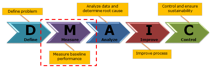
Six Sigma Phases

Six Sigma is a systematic problem-solving approach centered around defect elimination and variation reduction, leading to process improvement.

One of the principal tools in Six Sigma is the use of the DMAIC methodology. (Also see DMAIC Overview). Particularly, DMAIC is a logical framework that helps you think through and plan improvements to a process to achieve a Six Sigma level of excellence.

There are five phases that are used in the DMAIC method.

The purpose of the Measure phase is to understand the extent of the problem with the help of data. In other words, measure the process performance in its current state in order to understand the problem.

Goals of Measure Phase

• Establish baseline performance of the process
• Identification of process performance indicators
• Develop a data collection plan and then collect data.
• Validating the measurement system
• Determine the process capability

Measure Phase of DMAIC Overview

The Measure phase is approximately 2 to 3 weeks process based on the project inputs. In particular, all the relevant stakeholders’ involvement is key to getting quality data.

The measure phase is about the baseline of the current process, data collection, validating the measurement system, and determining the process capability. Multiple tools and concepts are available in the Measure phase of Six Sigma.

Process Definition & Basic Tools

Process map: A process map is a tool that graphically shows the inputs, actions, and also outputs of a process in a clear, step-by-step map of the process. 

The process map illustrates the relationship between inputs (X) and outputs (Y). Firstly, create a process map of all the activities required to convert raw materials into output (Y). Then, identify the Critical to Quality (CTQ) factors in the process.

Process map helps to identify the inefficiencies or wastes in the process. This also helps to determine the critical steps to collect the data.

Value stream mapping: Value stream mapping provides a visual representation of the organization’s flow of materials and information. Value stream mapping constitutes all the value-added and non-added values required to make the product. It consists of the process flows starting from the raw materials to making the product finally available in the hands of the customers.

Spaghetti Diagram: The spaghetti diagram, also known as the spaghetti chart, represents the basic flow of people, products, and process documents or papers.

Cause and Effect Matrix: The cause and effect matrix establishes the correlation between process input variables to the customer’s outputs during root cause analysis.

Data Collection

In fact, the measure phase is all about collecting as much data as possible to get the actual picture of the problem. Hence, the team must ensure the data collection measurement process is accurate and precise.

Data Types

Data is a set of values of qualitative or quantitative variables. It may be numbers, measurements, observations, or even just descriptions of things. Below are the types of Quantitative Data

• Discrete data: The data is discrete if the measurements are integers or counts. For example, the number of customer complaints, weekly defects data, etc.
• Continuous data: The data is continuous if the measurement takes on any value, usually within some range – for example, Stack height, distance, cycle time, etc.

Coding Data

Sometimes it is more efficient to code data by adding, subtracting, multiplying, or dividing by a factor.

Types of Data Coding

• Substitution – ex. Replace 1/8ths of an inch with + / 1 deviations from the center in integers.
• Truncation – ex. Data set of 0.5541, 0.5542, 0.5547 – you might just remove the 0.554 portions.

Data Collection Plan

A data collection plan is a useful tool to focus your data collection efforts on. This directed approach helps to avoid locating & measuring data just for the sake of doing so.

• Identify data collection goals
• Develop operational definitions
• Create a sampling plan
• Select & validate data collection methods

Plan for and begin collecting data

• Data collection form: In general, a data collection form is a way of recording the approach to obtaining the data that need to perform the analysis. Additionally, the data should be recorded by trained operators with a calibrated instrument and a standard data collection form.

• Data Collection check sheets: A Check Sheet is a data collection tool that usually identifies where and how often problems appear in a product or service. It’s specifically designed for the kind of process being investigated. 

Measurement System Analysis

Measurement System Analysis (MSA) is an experimental and mathematical method of determining how much variation within the measurement process contributes to overall process variability.

Accuracy: It is the difference between the true average and the observed average. If the average value differs from the true average, this is an indication of an inaccurate system.

Precision: Precision refers to how close the data points fall in relation to each other. In other words, a high-precision process will have little variance between the individual measurement points.

Gage R&R

The Gage Repeatability and Reproducibility is a method to assess the measurement system’s repeatability and reproducibility. Furthermore, Gage R&R measures the amount of variability in measurements caused by the measurement system itself.

Gage R&R focuses on two key aspects of measurement:

Repeatability: Repeatability is the variation between successive measurements of the same part, same characteristic, by the same person using the same gage.

Reproducibility: Reproducibility is the difference in the average of the measurements made by different people using the same instrument when measuring the identical characteristic on the same part.

Six Sigma Statistics

Basic Six Sigma statistics is the foundation for Six Sigma projects. It allows us to numerically describe the data that characterizes the process Xs and Ys. 

Statistics is the science of gathering, classifying, arranging, analyzing, interpreting, and presenting numerical data to make inferences about the population from the sample drawn. There are basically two categories – Analytical (aka Inferential statistics) and Descriptive (aka Enumerative statistics).

Inferential statistics: It is used to determine whether a particular sample or test outcome is representative of the population from the sample originally drawn.

Descriptive statistics: A descriptive statistic is basically organizing and summarizing the data using numbers and graphs. Descriptive statics is to describe the characteristics of the sample or population.

• Measure of frequency (Count, percentage, frequency)
• The measure of central tendency (Mean, median, mode)
• Measure of dispersion or variation (Range, variation, standard deviation)

The shape of data distribution is depicted by its number of peaks and symmetry possession, skewness, or uniformity. Skewness is a measure of the lack of symmetry. In other words, skewness is the measure of how much the probability distribution of a random variable deviates from the Normal Distribution.

Data Organization / Data Display / Data Patterns

The graphical analysis creates pictures of the data, which will help to understand the patterns and also the correlation between process parameters. Moreover, graphical analysis is the starting point for any problem-solving method. Hence select the right tool to identify the data patterns and display the data.

• Control Chart: The control chart is a graphical display of quality characteristics that have been measured or computed from a sample versus the sample number or time.
• Frequency Plots: Frequency plots allow you to summarize lots of data in a graphical manner making it easy to see the distribution of that data and process capability, especially when compared to specifications.
• Box Plot: A box plot is a pictorial representation of continuous data. In other words, the Box plot shows the maximum, minimum, median, interquartile range Q1, Q3, and outlier.
• Main Effects plot: The main effects plot is the simplest graphical tool to determine the relative impact of various inputs on the output of interest.
• Histogram: Histogram is the graphical representation of a frequency distribution. In fact, it is in the form of a rectangle with class intervals as bases and the corresponding frequencies as heights.
• Scatter plot: A Scatter Analysis is used when you need to compare two data sets against each other to determine a relationship.
• Pareto Chart: Pareto chart is a graphical tool to map and grade business process problems from the most recurrent to the least frequent.

Basic Probability & Hypothesis tests

Basic Six Sigma Probability terms like independence, mutually exclusive, compound events, and more are the necessary foundations for statistical analysis.

Additive law: Additive law is the probability of the union of two events. There are two scenarios in additive law:

• When events are not mutually exclusive
• When events are mutually exclusive

Multiplication law: It is a method to find the probability of events occurring simultaneously. There are two scenarios in multiplication law:

• When events are not independent
• When events are dependent

Compound Event: It is an event that has more than one possible outcome of an experiment. In other words, compound events are composed of two or more events.

Independent Event: Events can be independent events when the outcome of one event does not influence another event’s outcome. 

Hypothesis Testing

Hypothesis testing is a key procedure in inferential statistics used to make statistical decisions using experimental data. It is basically an assumption that we make about the population parameter.

When using hypothesis testing, we create:

• A null hypothesis (H0): the assumption that the experimental results are due to chance alone; nothing (from 6M) influenced our results.
• An alternative hypothesis (Ha): we expect to find a particular outcome.

Determine the process capability

Process Capability Analysis tells us how well a process meets a set of specification limits based on a sample of data taken from a process. The process capability study helps to establish the process baseline and measure the future state performance. Revisit the operational definitions and specify what are defects and which are opportunities.

Calculate the baseline process sigma

The value in making a sigma calculation is that it abstracts your level of quality enough so that you can compare levels of quality across different fields (and different distributions.) In other words, the sigma value (or even DPMO) is a universal metric that can help you with the industry benchmark/competitors.

Baseline Sigma for discrete data

Calculate the process capability through the number of defects per opportunity. The acceptable number to achieve Six Sigma is 3.4 Defects Per Million Opportunities (DPMO).

• DPO = Defects/(Units * Opportunity)
• DPMO =(Defects / Units * Opportunities) * Total 1,000,000
• Yield = 1-DPO (It is the ability of the process to produce defect-free units).

Baseline Sigma for Continuous data

Process Capability is the determination of the adequacy of the process concerning the customer needs. Process capability compares the output of an in-control process to the specification limits.  Cp and Cpk are considered short-term potential capability measures for a process.

Cpk is a measure to show how many standard deviations the specification limits are from the center of the process. 

• C_plower = (Process Mean – LSL)/(3*Standard Deviation)
• C_pupper = (USL – Process Mean)/(3*Standard Deviation)
• Cpk is the smallest value of the Cpl or Cpu:  C_pk= Min (C_pl, C_pu)

Six Sigma derives from the normal or bell curve in statistics, where each interval indicates one sigma or one standard deviation. Moreover, Sigma is a statistical term that refers to the standard deviation of a process about its mean. In a normally distributed process, 99.73% of measurement will fall within ±3σ, and 99.99932% will fall within ±4.5σ.

Measure Phase of DMAIC Deliverables

• Detailed process map
• Data collection plan and collected data
• Results of Measurement system analysis
• Graphical analysis of data
• Process capability and sigma baseline

Measure Phase of DMAIC Videos