

Attribute agreement analysis is how you test a measurement system whose output is a category instead of a number: pass or fail, go or no-go, good, rework or scrap. When people (or a vision system) make those calls, the question is whether they make them consistently and correctly. Attribute agreement analysis answers that with agreement percentages and the kappa statistic.
This guide covers what the study measures, why raw percent agreement can fool you, how to calculate Cohen’s kappa for two raters and Fleiss’ kappa for three or more (with a fully worked example of each), how to read the results, and how to design a study that tells you something useful. It finishes with the mistakes that show up again and again on the shop floor, plus practice questions.
A note on exams first. The ASQ Certified Six Sigma Green Belt body of knowledge lists percent agreement among the measurement system analysis tools (section III.E). The Black Belt body of knowledge lists percent agreement and an audit MSA for attribute measurement systems (V.C.1). The IASSC outlines list “Variable & Attribute MSA” (2.3.4) at Yellow, Green and Black Belt. None of them name kappa directly, but kappa is the statistic behind attribute agreement output in Minitab and other packages, and exam questions do ask about it.
What Is Attribute Agreement Analysis?
Every measurement systems analysis asks the same thing: how much of the variation in your data comes from the measurement process instead of the product? For a caliper or a CMM you answer with a variables Gage R&R study, which splits variance into repeatability and reproducibility. A visual inspector who sorts parts into “accept” and “reject” produces no standard deviation to split. So you look at agreement instead.
You use attribute agreement analysis whenever the result of a check is attribute (discrete) data on a nominal or ordinal scale. Typical cases:
- Visual inspection of welds, paint, castings, molded parts or printed labels (pass/fail).
- Go/no-go gages, where the gage gives a binary answer even though the feature is continuous.
- Defect classification: which of five defect codes applies, or whether a defect is critical, major or minor.
- Transactional judgments: whether an invoice is coded correctly, whether a call met the script, which category a customer complaint belongs to.
- Automated inspection, where a vision system is one of the “appraisers” and is compared with expert judgment.
Many references call the same study an attribute gage R&R or an attribute MSA. The names are used interchangeably in practice (see the FAQ for one exception).
A Pop-Culture Version: Umpires and the Strike Zone
A home plate umpire is an attribute measurement system. Every pitch gets a category, ball or strike, and nobody measures the result to the millimeter. Television broadcasts overlay a pitch-tracking box, which acts as the “known standard.” Fans then run an informal attribute agreement analysis every game: does this umpire call the same pitch the same way in the first inning and the ninth (repeatability)? Do two umpires agree on the same pitch (reproducibility)? Does the umpire agree with the tracking box (accuracy against the standard)? And the real complaint, when it comes, is rarely about one call. It is about a zone that drifts, which is exactly what a low within-appraiser agreement shows.
The same thing happens if you have ever culled a day of wildlife photos with a partner, each of you marking frames “sharp” or “soft.” The disagreements cluster on the borderline frames, and that is where an inspection study’s disagreements cluster too.
Attribute Agreement Analysis vs Variables Gage R&R
| Variables Gage R&R | Attribute agreement analysis | |
|---|---|---|
| Data | Continuous measurements (mm, psi, seconds) | Categories (pass/fail, defect codes, ratings) |
| Repeatability means | Equipment variation: spread of repeat readings by one appraiser | Within-appraiser agreement: does one appraiser give the same call on repeat trials? |
| Reproducibility means | Appraiser variation: difference between appraisers’ averages | Between-appraiser agreement: do different appraisers give the same call? |
| Accuracy check | Bias and linearity, studied separately | Each appraiser vs a known standard, inside the same study |
| Main statistics | %Study Variation, %Contribution, %Tolerance, ndc | Percent agreement, kappa, miss rate, false alarm rate (Kendall’s coefficients for ordinal ratings) |
| Information per reading | High | Low, so you need more parts for the same confidence |
One practical rule: if the characteristic can be measured on a continuous scale, measure it and run a variables study. A go/no-go gage on a diameter throws away information you could have had with a micrometer. Attribute agreement analysis is for judgments that really are categorical, or for checking the attribute inspection you are stuck with until a better gage arrives.
The Four Questions an Attribute Agreement Study Answers
A full study has each appraiser judge the same set of parts at least twice, in random order, without knowing which part is which. An expert, or a better measurement method, decides the correct answer for each part in advance: the known standard, sometimes called the master or reference value. With that data you can answer four questions.
- Within appraiser (repeatability): for what percentage of parts did each appraiser give the same answer on every trial? An appraiser who disagrees with themselves has no stable criterion.
- Each appraiser vs standard (accuracy): for what percentage of parts did each appraiser get every trial right? This is the number that tells you whether bad product is escaping, and through whom.
- Between appraisers (reproducibility): for what percentage of parts did all appraisers agree with each other on every trial? It can be high while everyone is wrong, if they all share the same mistaken criterion.
- All appraisers vs standard (overall effectiveness of the system): for what percentage of parts was every rating by every appraiser correct?
For pass/fail inspection, two more numbers matter for each appraiser, because the two kinds of error have very different costs:
- Miss rate: the share of ratings on truly bad parts that were called good. These are escapes to your customer.
- False alarm rate: the share of ratings on truly good parts that were called bad. These cost you scrap, rework and arguments with production.
These map onto the Type II and Type I errors of hypothesis testing, viewed from the null hypothesis that the part is good.
A Small Worked Study: Three Inspectors, Twelve Parts
Three inspectors (Ana, Ben and Cal) each judge 12 stamped brackets twice, pass or fail, in a different random order each trial. A quality engineer has already measured every bracket and set the standard: 8 good, 4 bad. Twelve parts is too few for a real study (more on that below); it keeps the arithmetic visible.
| Appraiser | Within appraiser | Vs standard | Miss rate | False alarm rate |
|---|---|---|---|---|
| Ana | 12 of 12 (100%) | 12 of 12 (100%) | 0 of 8 (0%) | 0 of 16 (0%) |
| Ben | 10 of 12 (83.3%) | 10 of 12 (83.3%) | 1 of 8 (12.5%) | 1 of 16 (6.3%) |
| Cal | 10 of 12 (83.3%) | 9 of 12 (75.0%) | 2 of 8 (25.0%) | 2 of 16 (12.5%) |
Across all three inspectors, all six ratings agreed on 7 of the 12 parts (58.3%), and on those same 7 parts every rating matched the standard, so all appraisers vs standard is also 58.3%. The story is clear even in a small study: Ana is applying the standard, Cal is letting bad brackets through, and the system as a whole is only as good as whoever is on shift. The fix is not more inspection. It is finding out what Ana looks at that Cal does not.
The site’s Gage R&R article has another percent-agreement example with a downloadable template and the Minitab menu steps for an attribute agreement analysis.
Why Percent Agreement Isn’t Enough
Percent agreement is easy to explain, and it is what the ASQ bodies of knowledge name. Its weakness is that some agreement happens by luck. Two inspectors who pass nearly everything will agree most of the time even if neither one looks at the parts.
Here is the extreme case. Your process makes 95% good parts. Two inspectors each flip a coin weighted to say “pass” 95% of the time. Their calls are pure noise, yet they agree whenever both say pass (0.95 x 0.95 = 0.9025) or both say fail (0.05 x 0.05 = 0.0025): 90.5% of the time. A 90% agreement figure from a study full of good parts can mean almost nothing.
That is the problem kappa solves. It asks how much better than chance the agreement is, as a share of the most improvement over chance that was possible.
Cohen’s Kappa for Two Raters
Jacob Cohen introduced kappa in 1960 for two raters classifying the same items into the same nominal categories. The formula:
kappa = (Po – Pe) / (1 – Pe)
- Po is the observed proportion of agreement: the share of items both raters put in the same category.
- Pe is the proportion of agreement expected by chance, given how often each rater uses each category: for each category, multiply rater A’s proportion by rater B’s proportion, then add across categories.
Kappa is 1 for perfect agreement and 0 when agreement is exactly what chance would give. It can go negative when raters agree less often than chance, which in practice usually means something is broken, such as one rater using the categories backwards.
Worked Example: Two Weld Inspectors
A fabrication shop wants to know whether its two weld inspectors apply the visual acceptance criteria the same way. Each inspects the same 50 welds independently and calls each one pass or fail.
| Inspector B: pass | Inspector B: fail | Total | |
|---|---|---|---|
| Inspector A: pass | 30 | 4 | 34 |
| Inspector A: fail | 6 | 10 | 16 |
| Total | 36 | 14 | 50 |
Step 1: observed agreement. They agree on 30 + 10 = 40 welds. Po = 40 / 50 = 0.80.
Step 2: chance agreement. A passes 34 / 50 = 0.68 of welds and B passes 36 / 50 = 0.72. If they were guessing at those rates, they would both say pass 0.68 x 0.72 = 0.4896 of the time, and both say fail 0.32 x 0.28 = 0.0896 of the time. Pe = 0.4896 + 0.0896 = 0.5792.
Step 3: kappa. kappa = (0.80 – 0.5792) / (1 – 0.5792) = 0.2208 / 0.4208 = 0.52.
Reading the result. Eighty percent agreement sounds respectable. Kappa says the inspectors capture only about half of the agreement that was available beyond chance. On the usual scales that is moderate agreement, below the 0.75 that most attribute MSA guidance treats as good. The 10 welds they disagree on are the place to start: pull them, put both inspectors in front of them with the acceptance standard, and find out which criterion each one is using.
The numbers were calculated in Python with exact fractions (kappa = 138 / 263 = 0.5247) and cross-checked with the cohens_kappa function in the statsmodels library.
Fleiss’ Kappa for Three or More Raters
Cohen’s kappa handles exactly two raters. Joseph Fleiss published a version in 1971 for any fixed number of ratings per item, which is what most inspection studies need. It is what Minitab reports in its attribute agreement analysis output.
Set up the data as N items, each rated by n raters into k categories, and let nij be the number of raters who put item i in category j.
- Agreement on each item: Pi = [sum over j of nij(nij – 1)] / [n(n – 1)]. This is the share of rater pairs that agree on item i.
- Mean observed agreement: P-bar = the average of the Pi values.
- Category proportions: pj = (total ratings in category j) / (N x n).
- Chance agreement: Pe = sum of pj2.
- Kappa: kappa = (P-bar – Pe) / (1 – Pe).
One subtle difference: Fleiss’ chance term uses the pooled category proportions of all raters, while Cohen’s uses each rater’s own proportions. So Fleiss’ kappa with two raters is not exactly Cohen’s kappa. On the weld data above, Fleiss’ version gives 0.524 against Cohen’s 0.525. The gap is usually small, but it explains why two software packages can print slightly different numbers for the same two raters.
Worked Example: Three Inspectors Grading Castings
A foundry’s final inspection sorts each casting into one of three dispositions: accept, rework or scrap. Three inspectors each grade the same 10 castings once. The table shows how many of the three put each casting in each category.
| Casting | Accept | Rework | Scrap | Pi |
|---|---|---|---|---|
| 1 | 3 | 0 | 0 | 1 |
| 2 | 3 | 0 | 0 | 1 |
| 3 | 2 | 1 | 0 | 1/3 |
| 4 | 0 | 3 | 0 | 1 |
| 5 | 0 | 2 | 1 | 1/3 |
| 6 | 0 | 0 | 3 | 1 |
| 7 | 3 | 0 | 0 | 1 |
| 8 | 1 | 2 | 0 | 1/3 |
| 9 | 0 | 1 | 2 | 1/3 |
| 10 | 1 | 1 | 1 | 0 |
| Total | 13 | 10 | 7 |
Step 1: agreement on each casting. With n = 3 raters there are n(n – 1) = 6 ordered rater pairs. When all three agree (castings 1, 2, 4, 6 and 7), the numerator is 3 x 2 = 6, so Pi = 1. A 2-to-1 split gives 2 x 1 = 2, so Pi = 2/6 = 1/3. A three-way split (casting 10) gives 0.
Step 2: mean observed agreement. P-bar = (5 x 1 + 4 x 1/3 + 0) / 10 = 6.333 / 10 = 0.633.
Step 3: chance agreement. There are 30 ratings in total. paccept = 13/30 = 0.433, prework = 10/30 = 0.333 and pscrap = 7/30 = 0.233. Pe = 0.4332 + 0.3332 + 0.2332 = 0.1878 + 0.1111 + 0.0544 = 0.353.
Step 4: kappa. kappa = (0.633 – 0.353) / (1 – 0.353) = 0.280 / 0.647 = 0.43.
Reading the result. The three inspectors agree unanimously on only half the castings, and kappa of 0.43 sits just above the 0.40 line that common guidance treats as poor. Look at where the splits fall: castings 3, 5, 8 and 9 are all one-step disagreements (accept vs rework, rework vs scrap), which points to a fuzzy boundary between adjacent categories rather than random calls. Boundary samples for each disposition, photographed and kept at the inspection station, are the usual first fix.
Calculated in Python with exact fractions (kappa = 42 / 97 = 0.4330) and cross-checked with the fleiss_kappa function in statsmodels.
Because these categories are ordered (accept is better than rework, which is better than scrap), kappa treats an accept vs scrap disagreement as no worse than accept vs rework. For ordinal ratings, Minitab also reports Kendall’s coefficient of concordance, which gives credit for near misses, and its documentation says Kendall’s coefficients are usually more appropriate when the categories are ordered.
How to Interpret Kappa
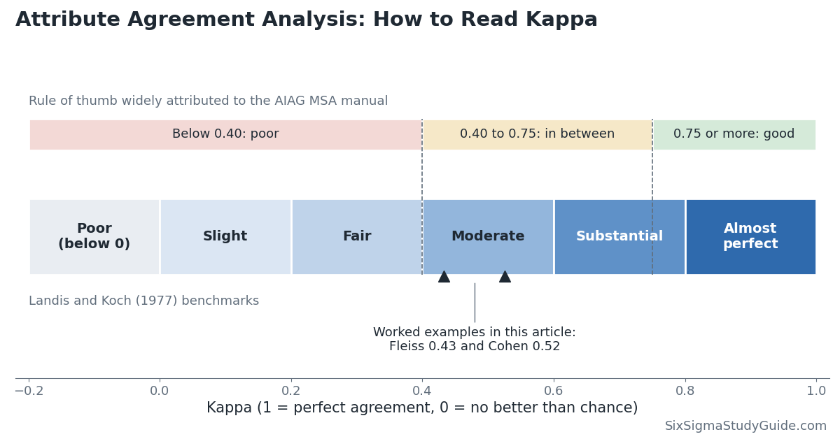
There is no law of nature that says what kappa is “good enough.” The bands you will see are conventions, and it is worth knowing where each one comes from.
Landis and Koch (1977). In a paper in the journal Biometrics, J. Richard Landis and Gary Koch proposed labels for ranges of kappa, while calling the divisions arbitrary. They are the most quoted scale in statistics and medical research, and they are the source of the “almost perfect agreement” wording exam questions use.
| Kappa | Landis and Koch label |
|---|---|
| Below 0 | Poor |
| 0.00 to 0.20 | Slight |
| 0.21 to 0.40 | Fair |
| 0.41 to 0.60 | Moderate |
| 0.61 to 0.80 | Substantial |
| 0.81 to 1.00 | Almost perfect |
The AIAG guideline. In manufacturing, especially automotive, the rule of thumb is that kappa above 0.75 indicates good agreement and kappa below 0.40 indicates poor agreement, attributed to the AIAG Measurement Systems Analysis reference manual. Minitab’s documentation repeats the 0.75 figure and adds that larger values, such as 0.90, are preferred. Many customers set 0.90 for critical characteristics.
Effectiveness, miss rate and false alarm rate. For pass/fail studies against a standard, the same automotive guidance is usually summarized as below. Treat it the same way: a widely used convention that your customer may tighten.
| Decision | Effectiveness | Miss rate | False alarm rate |
|---|---|---|---|
| Acceptable | 90% or more | 2% or less | 5% or less |
| Marginal, may need improvement | 80% or more | 5% or less | 10% or less |
| Unacceptable | Below 80% | Above 5% | Above 10% |
A few more points that matter when you read real output:
- Ignore the p-value on its own. Software tests whether kappa is greater than zero. Almost any trained inspector beats chance, so a significant p-value tells you very little. The size of kappa is what matters.
- Look at kappa by category. Minitab reports kappa for each response category as well as overall. A low kappa for “scrap” with a high one for “accept” tells you exactly which boundary to work on.
- Kappa depends on the mix of parts. When almost every part is good, Pe is high and a few disagreements pull kappa down sharply, even while percent agreement stays above 90%. This is sometimes called the kappa paradox. It is a property of the study, not a flaw in the inspectors, which is why the study design below insists on a real mix of good and bad parts.
- Small studies give wide uncertainty. Minitab shows confidence intervals on the percent agreement figures. With 12 parts, as in the small worked study, a 75% result could easily come from an inspector whose long-run rate is much higher or lower.
How to Design an Attribute Agreement Study
Most bad attribute agreement analysis results come from the study design, not the statistics. A good design looks like this.
- Write the operational definition first. If the acceptance criterion is “no excessive porosity,” the study will only measure how differently people read “excessive.” Define the categories in words, with photos or physical boundary samples, before you test anyone against them.
- Use enough parts. Attribute data carries little information per rating, so attribute studies need more parts than the 10 typical of a variables Gage R&R. Common practical guidance is 30 to 50 parts or more, and more when the categories are many or the consequences of a miss are serious. No single number is mandated; size the study to how precise you need the answer to be.
- Choose the mix of parts on purpose. Do not pull a random sample of production; at a 99% yield you would get almost no bad parts. Include clearly good parts, clearly bad parts and a meaningful share of borderline parts on both sides of the limit. Many practitioners aim for something close to half good and half bad, with the borderline parts doing most of the work. Every category you want to test must appear several times.
- Set the standard independently. The known standard should come from a better method than the one under test: a measurement, a destructive test, or a consensus of experts who are not appraisers in the study.
- Use the people who do the job. Two to three appraisers who normally make the call, under normal lighting, time pressure and tools. Testing the quality engineer instead of the second-shift inspector tells you about the wrong measurement system.
- Keep it blind and randomized. Label parts with codes only the study owner can decode, present them in a new random order on each trial, and separate trials in time so appraisers cannot remember their earlier answers. Appraisers should not see each other’s ratings or the standard.
- Run at least two trials. Without repeats you cannot measure within-appraiser agreement. Two or three trials are typical.
- Record everything, including comments. When an appraiser says “I wasn’t sure about this one,” write it down. Those notes point straight at the unclear part of the definition.
Common Mistakes
- Reporting percent agreement alone on a study dominated by good parts, and calling 92% “acceptable.”
- Judging only between-appraiser agreement with no standard. Inspectors can agree perfectly and all be wrong.
- Using obvious parts only. A study of clearly good and clearly scrap parts gives a flattering kappa and says nothing about the borderline, which is where the real decisions are made.
- Letting appraisers recognize the parts, for example by a memorable scratch or a visible part number, so trial 2 becomes a memory test.
- Using Cohen’s kappa for more than two raters, or averaging pairwise Cohen’s kappas and calling the result Fleiss’ kappa. They are different statistics.
- Using kappa on ordered ratings without also looking at Kendall’s coefficients, which treat a one-step disagreement differently from a three-step one.
- Running the study once and never again. New inspectors, new defect types and drifting standards all degrade agreement over time.
Attribute Agreement Analysis in Practice
In a DMAIC project, attribute agreement analysis belongs in the Measure phase, before you trust any defect data. If the project’s baseline is “6% of welds rejected,” and the two inspectors who made those rejections have a kappa of 0.52, the baseline is partly a measure of who was on shift. Fix the measurement system first, or your improvement will be judged by the same noisy yardstick.
Here is how a practitioner typically works through it.
- Start with the disagreements, not the summary. Sort the parts by how much the ratings split. The few parts that cause most of the disagreement are your Pareto of measurement problems.
- Bring the appraisers together over those parts. Ask each person what they looked at. Usually you discover two criteria in use (one inspector rejects any visible spatter, another only spatter on the sealing face), or a defect that is hard to see under the station’s lighting.
- Fix the system, not the person. Rewrite the definition, build a boundary sample board, improve lighting or magnification, add a simple fixture or a poka-yoke. Retraining alone fades quickly if the standard stays vague.
- Rerun the study with fresh parts and compare kappa and miss rate before and after. That before-and-after comparison is a measurable project win in its own right.
- Consider replacing the judgment. If agreement stays poor after a real effort, ask whether the characteristic could be measured with a variables gage. A continuous measurement is almost always a better measurement system than a human category.
The same approach works away from the factory. Claims processors coding the reason for a denial, nurses scoring a triage category, or auditors rating a call as compliant are all attribute measurement systems. Downstream, the counts they produce feed attribute control charts and capability figures, so poor agreement quietly corrupts everything built on top of it.
Attribute Agreement Analysis Practice Questions
Question 1
Two appraisers classify the same parts. Their observed agreement is 0.90, and the agreement expected by chance is 0.60. What is Cohen’s kappa?
(A) 0.30
(B) 0.50
(C) 0.75
(D) 0.90
Answer: (C) 0.75. kappa = (0.90 – 0.60) / (1 – 0.60) = 0.30 / 0.40 = 0.75. Choice (A) is only the numerator, and (D) is the raw percent agreement, which ignores chance.
Question 2
Four inspectors each classify the same 40 circuit boards into one of three defect categories. Which statistic best measures how well the inspectors agree with each other beyond chance?
(A) Cohen’s kappa
(B) Fleiss’ kappa
(C) %Study Variation
(D) Pearson correlation coefficient
Answer: (B) Fleiss’ kappa. Cohen’s kappa is defined for exactly two raters. %Study Variation belongs to variables Gage R&R, and a correlation coefficient needs numeric data. If the three categories were ordered by severity, Kendall’s coefficient of concordance would be worth reporting alongside it.
Question 3
Two inspectors check 100 parts. Both pass 92, both fail 3, inspector A passes 3 that B fails, and B passes 2 that A fails. They agree on 95% of parts. What is Cohen’s kappa, to two decimals?
(A) 0.52
(B) 0.75
(C) 0.90
(D) 0.95
Answer: (A) 0.52. Po = 0.95. A passes 95 parts and B passes 94, so Pe = 0.95 x 0.94 + 0.05 x 0.06 = 0.893 + 0.003 = 0.896. kappa = (0.95 – 0.896) / (1 – 0.896) = 0.054 / 0.104 = 0.52. With so few bad parts, chance agreement is already very high, so 95% agreement translates into only moderate kappa. It is also a sign the study needed more bad and borderline parts.
Attribute Agreement Analysis FAQ
What is a good kappa value?
By the common manufacturing rule of thumb, 0.75 or more is good, 0.90 or more is preferred, and below 0.40 is poor. On the Landis and Koch scale, above 0.80 is “almost perfect.” Both are conventions. Check whether your customer or industry sets its own limit, and set a stricter one for safety-critical calls.
What is the difference between Cohen’s and Fleiss’ kappa?
Cohen’s kappa compares exactly two raters, and its chance term uses each rater’s own category rates. Fleiss’ kappa works for any fixed number of ratings per item and uses the pooled category rates of all raters. With two raters they give close but not identical answers.
Is attribute agreement analysis the same as attribute gage R&R?
In everyday use, yes. Both names describe a study of repeatability, reproducibility and accuracy for a categorical measurement system. Some references reserve “attribute gage study” for a different method, the analytic method, which estimates bias and repeatability of a go/no-go gage from parts with known reference values. If a customer asks for an “attribute gage R&R,” confirm which one they mean.
How many parts do I need for an attribute agreement analysis?
More than for a variables study. Common guidance is 30 to 50 parts or more, with a deliberate mix of good, bad and borderline parts and two or three trials per appraiser. The right number depends on how precise the answer has to be, so look at the confidence intervals your software reports and add parts if they are too wide to support a decision.
Related Pages
- Measurement systems analysis (MSA)
- Gage repeatability and reproducibility (GR&R)
- Evaluating the measurement process (EMP studies)
- Types of data and scales of measurement
- Attribute control charts
When you’re ready, there are a few ways I can help:
First, join 12,000+ other Six Sigma professionals by subscribing to my email newsletter. A short read every Monday to start your work week off correctly. Always free.
* * *
If you’re looking to pass your Six Sigma Green Belt or Black Belt exams, I’d recommend starting with my affordable study guide:
1)→ 🟢Pass Your Six Sigma Green Belt: a study guide organized by the exam Body of Knowledge, 1,000+ practice questions with detailed answer explanations, and 15+ full-length mock exams
2)→ ⚫Pass Your Six Sigma Black Belt: the full Black Belt Body of Knowledge, 2,000+ practice questions with detailed answer explanations, and 15+ full-length mock exams
You’ve spent so much effort learning Lean Six Sigma. Why leave passing your certification exam up to chance? This comprehensive study guide offers 1,000+ exam-like questions for Green Belts (2,000+ for Black Belts) with full answer walkthroughs, access to instructors, detailed study material, and more.
Thousands have used this system to prepare. Join them here.