What is a Cumulative Sum Chart?

A cumulative sum chart (CUSUM) is a type of control chart used to detect the deviation of the individual values or subgroup mean from the adjusted target value. In other words, monitor the deviation from the target value. CUSUM chart is an alternative to Shewhart control charts.

The basic advantage of the CUSUM chart is that it is more sensitive to the small shift of the process means when compared to the Shewhart charts (Individuals I-MR or Xbar charts).”

The cumulative sum chart and the exponentially weighted moving average (EWMA) charts also monitor the mean of the process, but the basic difference is unlike Xbar charts. They consider the previous value means at each point. Moreover, these charts are considered a reliable estimate when the correct standard deviation exists.

When Would You Use a Cumulative Sum Chart?

The purpose of the CUSUM chart is to monitor the small shift in the process mean of the samples collected at time intervals. These measurements of samples at a given time interval represent the subgroups.

Instead of calculating the subgroup’s mean independently, the CUSUM chart represents the information from current and previous samples. Hence, the CUSUM chart is always better than the Xbar charts in detecting the small shifts of process mean. The CUSUM chart is more effective when the sample size is one. These charts are basically used in process industries and in manufacturing.

Comparison between CUSUM and Shewhart chart

The purpose of the CUSUM and Shewhart charts is to detect the mean shifts in the process; the basic differences are:

• CUSUM charts consider all the samples up to a current point and also consider the current sample for measurement, whereas the Shewhart chart is based on the single subgroup measurement.
• The determination of the out-of-control limit in CUSUM charts is based on the decision interval or the use of the V-Mask method, whereas the Shewhart chart is based on control limits (upper and lower control limits).
• CUSUM charts’ control limits are computed from average run length specs, whereas the Shewhart chart control limits are generally at the three-sigma limits.

Advantages of the CUSUM chart

• CUSUM charts are the best way to detect the small shifts in process mean, especially 0.5 to 2 SD from the target mean.
• It is easy to identify the shifts in the process visually.

Disadvantages of the CUSUM chart

• Establishing and maintaining CUSUM charts is more complicated.
• CUSUM charts are slower in detecting large process mean shifts.
• Since CUSUMs are correlated, it is tough to interpret the patterns.

How do you make a Cumulative Sum Chart?

The CUSUM charts can be represented in the visual method, i.e., V-mask. This method was introduced by Barnard in 1959 to check whether a process is out of control or not. Still, the generally tabular (algorithmic) method will be used to monitor the process. Unlike other standard control charts, all previous measurements for CUSUM charts are included in the calculation for the latest plot. But, establishing and maintaining the CUSUM is difficult.

V-Mask Method

V-mask looks like a sideways V. The V-mask chart checks whether each marked sample falls within the boundaries of the V-mark. If any point falls outside of the control limit, that indicates a signal mean shift in the process. When each sample is plotted, the V-mask may have shifted to the right. The below graph shows the V-mask and related formulas.

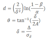
The behavior of the V-Mask is determined by the distance k (which is the slope of the lower arm) and the rise distance h. The team could also specify d and the vertex angle (or, as is more common in the literature, q = 1/2 the vertex angle). For an alpha and beta design approach, we must specify

• α, the probability of concluding that a shift in the process has occurred, when in fact, it did not. 
• β, the probability of not detecting that a shift in the process mean has, in fact, occurred.
• δ (delta), the detection level for a shift in the process mean, expressed as a multiple of the standard deviation of the data points.

Tabular Method

The Tabular method is an easier method than the V-Mask method. Here are the steps to make a CUSUM chart.

• First of all, estimate the standard deviation of the data from the moving range control chart σ= R̅/d₂.
• Calculate the reference value or allowable slack since the CUSUM chart monitors the small shifts. Generally, 0.5 to 1 sigma will be considered. K= 0.5 σ.
• Compute decision interval H, generally ± 4 σ will be considered (some place ± 5 σ also be used).
• Calculate the upper and lower CUSUM values for each individual i value.

• Upper CUSUM (UC_i)= Max[0, UC_i-1+x_i – Target value-k).

• Lower CUSUM (LC_i)= Min[0, LC_i-1+x_i – Target value+k).

• Draw all UC_i & LC_i values in the graph and also draw decision intervals (UCL and LCL).
• Check if any of the UC_i values are above the UCL and any of the LC_i values are below the LCL.
• Finally, take necessary action to eliminate the special causes if any of the points are out of control limits.

Calculate the plotting position

To find the plotting position for the new point in a cumulative sum chart, you can use the following formula.

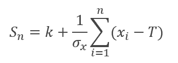
Where:

• S_n= Plotting Position
• k = reference value or the center line of the cumulative sum chart (if provided)
• x_i = The new point you want to plot
• T=Target value
• σ_x = Std Dev

Example: Find the plotting position for the new point 80 in the cumulative sum chart for the standard deviation 5, target value 70 and k=0.5.

To find the plotting position for the new point of 80 in a cumulative sum chart, you can use the following formula:

Plotting position = k + [(x_i – Target value) /σ]

Where:

k = 0.5 (the center line of the cumulative sum chart)

x_i = 80 (the new point you want to plot)

Target value = 70 (the target value for the process)

σ= 5 (the standard deviation of the process)

So,

Plotting position = 0.5 + [(80 – 70) / 5]

Plotting position = 0.5+2=2.5

Therefore, the plotting position for the new point of x_i = 80 in the cumulative sum chart is 2.5.

Example of Using a Cumulative Sum Chart in a DMAIC Project

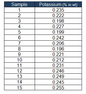
Example: CUSUM chart will be used in the control phase of DMAIC. In a drug manufacturing unit, potassium content is one of the important parameters. The target potassium content is 0.21% in wt. Therefore, the team has collected 25 batches from the production in a time interval to monitor the process mean shift.

Step1:

Estimate the standard deviation of the data from the moving range control chart σ= R̅/d₂.

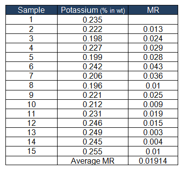
• n=2
• d2 = 1.128
• σ= R̅/d₂ = 0.01914/1.128 = 0.0169

Refer to common factors for various control charts.

Step 2:

Calculate the reference value or allowable slack K= 0.5 σ = 0.5*0.0169 = 0.00848

Step 3:

Compute decision interval H, generally ± 4 σ = ± 4 * 0.0169= ± 0.0679

UCL = +0.0679 and LCL = -0.00679

Step 4:

Calculate the upper and lower CUSUM values for each individual i value.

Target value =0.21

Upper CUSUM (UC_i)= Max[0, UC_i-1+x_i – Target value-k)

Lower CUSUM (LC_i)= Min[0, LC_i-1+x_i – Target value+k)

For the first sample: 0.235

• Upper CUSUM (UC₁)= Max[0, 0+0.235– 0.21-0.0084) =0.017
• Lower CUSUM (LC₁)= Min[0, 0+0.235-0.21+0.00848) = 0

For the second sample: 0.222

• Upper CUSUM (UC₁)= Max[0, 0.017+0.222– 0.21-0.0084) =0.02
• Lower CUSUM (LC₁)= Min[0, 0+0.0222-0.21+0.0084) = 0

Similarly, find the Upper and Lower CUSUM for all the samples:

Step 5:

Draw all UC_i & LC_i values in the graph and also draw the decision intervals (UCL and LCL).

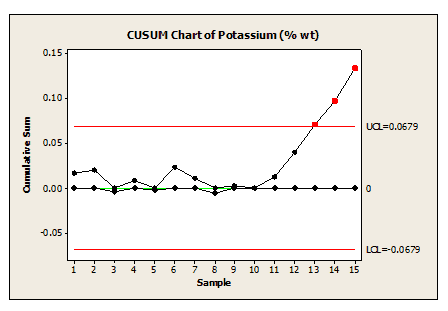
Step 6:

Conclusion: It is clearly evident from the above graph that from sample 13 onwards the process is going out of control. Hence, the team has to identify the special cause and take the appropriate corrective action.

Compare a CUSUM example with a Shewhart Chart.

Furthermore, use a sample example from the above and draw the Individual I-MR.

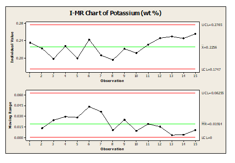
From the above graph, it is clearly evident that both the Individual and Moving range process is in control and predictable. Still, the sample example CUSUM chart shows the process is going out of control. Hence, CUSUM charts are more effective in monitoring the small shifts in the process mean than Individuals I-MR or Xbar charts.

What Do You Need to Know for Your Exam?

Green Belts

The IASSC Green Belt BOK requires you to know EWMAs as part of Statistical Process Control.

Black Belts

The Villanova Black Belt BOK notes you are required to “Understand appropriate uses of short-run SPC, EWMA, CuSum, and moving average.”

The IASSC Black Belt BOK lists CUSUM Charts under what’s needed for 5.2 Statistical Process Control (SPC).

Cumulative Sum Chart Videos

Helpful Links

• https://pdfs.semanticscholar.org/b941/60c2b0f01675879e8ea0378fe891d1399b35.pdf

When you’re ready, there are a few ways I can help:

First, join 30,000+ other Six Sigma professionals by subscribing to my email newsletter. A short read every Monday to start your work week off correctly. Always free.

—

If you’re looking to pass your Six Sigma Green Belt or Black Belt exams, I’d recommend starting with my affordable study guide:

1)→ 🟢Pass Your Six Sigma Green Belt​​

2)→ ⚫Pass Your Six Sigma Black Belt ​​​

You’ve spent so much effort learning Lean Six Sigma. Why leave passing your certification exam up to chance? This comprehensive study guide offers 1,000+ exam-like questions for Green Belts (2,000+ for Black Belts) with full answer walkthroughs, access to instructors, detailed study material, and more.

​ Join 10,000+ students here.