What is Central Tendency?

Central tendency refers to the statistical measure used to determine the center of a distribution of a data set. We also call it a measure of central location. In other words, the single value most represents the entire data set.

Central tendency reflects the principle that when using normal data, all three of the main measures (mean, mode, median) tend to be roughly the same.

When Do You Use It?

Central Tendency is the widely used method in basic data analysis. Based on the situation, the central tendency measure could be Mean, Median, or Mode.

Mean (Average)

The mean is a well-known measure of central tendency, and it is also the most commonly used method for measuring the center value of a continuous data set. The mean is the total of all data values divided by the number of data points, and it is also called the arithmetic mean. Different types of means exist: like the arithmetic mean, geometric mean, weighted mean, etc. The notation for the population mean is represented with μ (“Mu”), whereas the sample mean is represented as X̅.

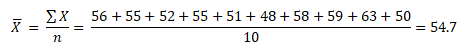
Where X represents each number and n is the sample size.

One advantage of the mean–you are not required to sort the data. Likewise, it uses all the data values for the calculations.

The disadvantage of the mean is that the data is influenced by outliers, and the mean is not the actual value of any data point.

Median

The median is the middle value when the data is arranged in ascending or descending order. If the data set has even values, then the median is the average of the middle two values.

An advantage of the median is it provides an idea of where most of the data is located, and also, it is not impacted by outliers.

A disadvantage is that the data must be sorted and arranged, and the median has more variation than mean

Mode

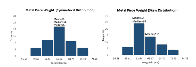
The mode is the value that occurs most often in the data set. It is possible for groups of data to have more than one mode if multiple numbers are tied for the greatest frequency in the data set. In the histogram, we can identify the mode with the highest bar.

An advantage of Mode is that there is no need to sort the data, unlike the median, and it is not influenced by outliers.

A disadvantage of Mode is sometimes it will have multiple modes, and a few times, no mode in the data set.

Notes about Central Tendency

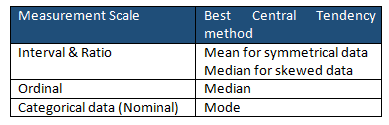
The most common assumption of a statistical test is that data is normally distributed. For normally distributed data, we can use any of the central tendency methods (mean, mode, or median) because, for symmetrical data, all three values are equal. However, most statisticians use the mean as it considers all the values in the data set for calculation, and if any value changes, it will affect the mean.

The median is the best central tendency method: as the skew increases, the difference between the mean and median will also increase.

A central tendency is rarely perfectly centered. Even if it was, it wouldn’t stay that way. As time goes on, a standard deviation can drift over 1.5 sigmas over time.

Without a 1.5 sigma drift, a 6 Sigma process would only generate 2 defects per BILLION! As it is, because of this drift, the errors are 3.4 per million.

Examples in DMAIC

Central Tendency is the widely used method in the Measure phase of DMAIC.

Example 1

Find the mean, median, and mode of weight distribution for a piece of metal.

Mean: What is the mean (average) weight of a metal piece (in gms)

56,55,52,55,51,48,58,59,63,50

Where N=10

Median: What is the median weight of a metal piece (in gms)?

56,55,52,55,51,48,58,59,63,50

Sort the data

48,50,51,52,55,55,56,58,59,63

Since N=10 (even number), average the two middle values = 55+55/2 = 55

Mode: What is the mode of the distribution of a metal piece (in gms)?

56,55,52,55,51,48,58,59,63,50

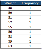
Since the frequency of the 55 weight is 2, therefor Mode of the weight distribution is 55.

Example 2

Find the cumulative frequency distributions using Central Tendency.

Mean, Median, and Mode of grouped data:

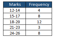
Since we don’t have exact marks for each individual, approximate Mean and Median values can be calculated using frequency distribution.

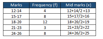
Find the mid marks of each class:

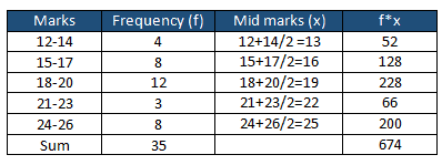
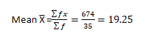
Multiply frequency with Mid marks:

Median

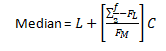
• Where L is the lower boundary of median class
• F_L = Cumulative frequency of lower class next to the median class
• F_M = Frequency of median class
• C = Class width

Find the cumulative frequency:

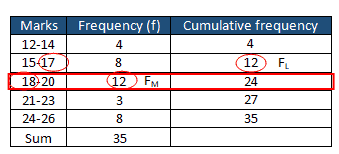
The sum of frequency Σf is 35, so Σf/2 =17.5

The smallest cumulative frequency greater than or equal to 17.5 is 24, and the corresponding median class is 18-20

The frequency of the median class is 12 (F_M) and the Cumulative frequency of the lower class next to the median class is 12 (F_L). When the data values are whole numbers, simply subtract 0.5 from the lower limit(18-0.5 =17.5) or add the first number from F_M row (18) and the last number from the previous row (17) and divide by two. i.e (18+17)/2 =17.5

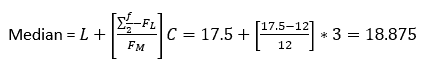
• L= =17.5
• F_L =12
• F_M =12
• C=14-12=3

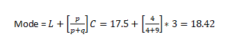
Mode

• p= highest frequency minus the frequency of the next lower class
• q= highest frequency minus the frequency of the next higher class

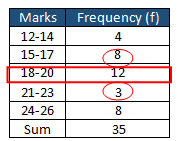
• p=12-8=4
• q=12-3=9

Videos on Central Tendency