When we use a sample group to gain insight into an entire population–whether we’re talking about people or a product built in a factory–we risk the sample group not completely reflecting the whole population. Therefore, we need confidence intervals.
Further, we use confidence intervals to calculate a degree of certainty that the sample group accurately represents the entire population from which they were drawn. Another way of thinking of it is that if you drew the same-sized sample group hundreds of times and performed the same measurements, a certain percentage of confidence intervals in those sample groups will contain the population means.
A confidence interval is a range of values. So, you can have a percentage of certainty that the population’s mean lies within that range in any given sample from that population.
Confidence Interval vs. Confidence Level
A confidence interval is a range of values that probably contain the population mean.
However, a confidence level is a percentage of certainty that, in any given sample, that confidence interval will contain the population mean.
Confidence Interval vs. Prediction Interval
Prediction intervals are used to calculate the next probable data point. They tell you about the distribution of data values, whereas confidence intervals tell you about a probable population mean.
Estimating Population Mean and Standard Deviation
In most cases, we won’t know the mean and standard deviation for an entire population. However, we can calculate the mean and standard deviation for each of our samples. So we can use the sample figures to estimate those of the whole population. This is what we call a point estimate.
Once we find the point estimate, we also need to know how accurate it is. For instance, the Central Limit Theorem says that in a large enough sample group (30 or more), the sample’s mean and standard deviation will be close to those of the population.
Margin of Error
The margin of error is the maximum expected difference between the actual population parameter and a sample estimate of the parameter. In other words, it is the range of values above and below sample statistics.
Margin of error widely used in surveys tells the degree of uncertainty that the survey results might have.
Margin of error = 1/√n
Where n= sample size
The margin of error is the product of the critical value and the standard error in the confidence interval. If the margin of error increases, the confidence level increases. Similarly, if the margin of error decreases, the confidence level also decreases.
For example, to estimate the confidence interval, we may use X̅±E
E is the margin of error.
Confidence interval = X̅±Zα/2*σ/√n
- Where σ = population standard deviation
- Zα/2 = normal distribution value for the desired confidence level
- n = sample size
- X̅ = sample mean
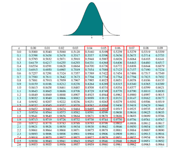
Z Scores
A Z score is the number of standard deviations between a data point and its mean. Thus, you can use a Z-score table to find the corresponding Z-score for common confidence levels or calculate the α value using this formula:
α = 1 - confidence level
If your desired confidence level is 95%, then your calculation would look like this:
α = (1 - 0.95)
α/2 = (1 - 0.95) / 2 = 0.025
Zα/2 = Z0.025 =1.96
Common confidence intervals and corresponding Z scores
| Desired Confidence Interval | Z Score |
| 90% | 1.645 |
| 95% | 1.96 |
| 99% | 2.576 |
Confidence Interval Question Using Z-Score
Question: We conduct a random survey of 500 newly-enrolled university students. We know that the standard deviation for university enrollment age is eight years. The mean age of our sample is 24. Calculate the confidence interval for all first-year university students with a 99% confidence level to 3 decimal places.
Calculation: The first step is to consult a Z-score table. A 99% confidence level requires a Z-score of 2.576.
Zα/2 = 2.576, X̅ = 24, σ = 8 and n = 500
Margin of error E = Zα/2*σ/√n = 2.576*8/√800 = 0.922
Confidence interval = X̅±Zα/2*σ/√n = 24±0.922
Answer: Hence, the confidence interval for the age of first-year university students is 23.07–24.922, with a 99% confidence level.
Confidence Interval Question Using T-Score
Question: A factory produces tennis balls. A sample of 19 balls is taken from one factory production day. The mean weight of the sample balls is 58.2g. The standard deviation for the sample balls is 0.4g. Calculate the confidence interval with a confidence level of 95%.
Calculation: The sample size is too small to use a Z-score. Instead, use a T-score, which uses a t-distribution. Finding a confidence interval for a mean is a two-tailed test.
You’ll need an alpha score. To calculate it, use this simple equation:
α = (100% - confidence level%)
α = (100% - 95%)
α = 5%
You also need the degrees of freedom (df), which is the number of samples minus one. Or in equation form:
df = n - 1
df for this question is 18.
So, use a T-table to look up the T-score needed for a two-tailed test with an α of 5% and a df of 18: the answer is 2.101.
tα/2=2.101, X̅=58.2, σ=0.4 and n=19
Margin of error E =tα/2*σ/√n = 2.101*0.4/√19 = 0.192
Confidence interval = X̅±tα/2*σ/√n = 58.2±0.192
Answer: Hence, a 95% confidence interval for tennis balls produced in the factory is 58.008–58.392g.
Calculating the Confidence Interval Comparing Two Population Means
Using samples from each population, you can also use confidence intervals to compare two population means. Use this method to compare two different manufacturing methods or to look for differences in two groups of people (for example, smokers and non-smokers). You could also use it to decide whether or not it will be acceptable to pool your two population samples into one larger sample.
The confidence interval for comparing two means is a range of values in which the difference between those two means might lie.
We use a similar equation to the one we use to calculate a population mean. Instead of looking for x, we’re looking for the difference between means.
Z = ((x̄1 - x̄2) – (x1 – x2)) / √((s12 / n1) + (s22 / n2))
Or, in a slightly easier-to-read format:

Example
High blood pressure has been causally linked to smoking tobacco products. To test this, you want to compare systolic blood pressure between smokers and nonsmokers. You’ll use a confidence level of 95%.
- You have 45 smokers and 56 non-smokers, with similar variance (age, gender, health levels) in each group.
- In the sample group of smokers, the mean systolic rate is 138.
- In the sample group of nonsmokers, the mean systolic rate is 135.
- The standard deviation for smokers is 16.5.
- The standard deviation for nonsmokers is 14.9.
- The Z-score you need is 1.96.
n1 = 45
n2 = 56
Z = 1.96 (found by looking up 95% confidence level on the chart.)
s1 = 16.5
s2 = 14.9
x̄1 = 138
x̄2 = 135

Confidence Interval=(x̄1 - x̄2)±Z*√((s12 /n1 )+(s22 /n2)
Firstly, plug the numbers into the equation, so our confidence interval, with a confidence level of 95%, is::
Confidence Interval=(x̄1 - x̄2)±Z*√((s12 /n1 )+(s22 /n2)
= (138 - 135) ± 1.96* √((16.52 / 45) + (14.92 / 56))
= (3)±1.96×√(10.014)
= (3)±1.96×3.16
= (3)±6.19
Confidence Interval≈(3−6.19,3+6.19)
≈ (−3.19,9.19)

To find the margin of error, use:
margin of error = Z * √((s12 / n1) + (s22 / n2))
margin of error = 1.96 * √((16.52 / 45) + (14.92 / 56))
margin of error = 1.96 * √((272.25 / 45) + (222.01 / 56))
margin of error = 1.96 *  √(6.05 + 3.9645)
margin of error = 6.2025

Therefore, the margin of error for the difference in means between smokers and nonsmokers, with a 95% confidence level, is 6.19. This means that we are 95% confident that the true difference in means falls within ±6.19 units of the sample difference.
Additional Confidence Intervals Videos
Confidence intervals for Variation
The point estimate for σ is s. s2 is the most unbiased estimate of σ2.
Use the chi-square distribution to construct a confidence interval for the variance and standard deviation
If the random variable x has the normal distribution, the distribution of:
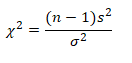
For sample size n > 1
Confidence intervals for variation:

Where n= sample size
s2 = point estimate of variance:

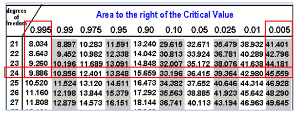
Example: XYZ pharmaceutical company randomly selected 25 samples of flu medicines. The sample variance is 6 milligrams. For instance, assume the weights are normally distributed and construct a 99% confidence interval for the population variance.
n=25
Degrees of freedom = n -1 = 24
s2 = 6
chi square α/2 = 45.55
chi square 1-α/2 = 9.886
Confidence intervals for variation:
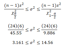
Hence, with 99% confidence, you can say that the population variance is between 3.161 and 14.56 milligrams.
Confidence intervals for Proportion
Central theorem says that with larger samples, every sample proportion will have a normal distribution. For larger sample sizes, sample size times proportion (np) and n (1-p) great than equal to 5, the normal distribution can be used to calculate the confidence interval for a proportion.
The confidence intervals for proportion is:
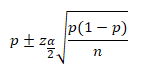
Where:
n=sample size
p= population proportion estimate
Zα/2 = appropriate confidence level from Z table
Example: In a bulb manufacturing unit, 24 defective bulbs were identified in a sample size of 400 bulbs. Calculate the 95% confidence interval for the proportion.
n=400
P = 24/400 = 0.06
1-p = 0.94
Zα/2 = 1.96 (95% confidence)
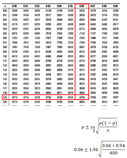
0.06±0.0232
0.036≤p≤0.083
So, with 95% confidence, the population proportion is between 0.036 and 0.083.
What is the Difference Between Control Limits and Confidence Intervals?
These are two entirely different concepts. One is used in the Analysis of a process, and the other in the Control of a process.
Further, Control limits depend on your population or sample’s distribution. They can be defined as the average + or – 3 standard deviations. “Control limits are obtained based on the nature of the distribution of data that you collect; if a process is in control doesn’t mean that your process is stable. Hence control limits give the limits at that instant.”
These are different from Specification limits which generally show up on control charts. They are assigned by businesses for what is viable for them. A colleague once described them as if the process goes above this level, we all must update our resumes. So, if it goes below this other limit, don’t worry about updating resumes; no one will ever hire us again!
Confidence Interval
Confidence intervals are a device of statistics for when you do not have perfect knowledge of all of the data. For example, imagine you are trying to infer the chance of some event happening by sampling from a population. Let’s take US voting polls. CNN can’t possibly get all of the voting data, but they can sample the population through exit polls. From that sample, they can predict the winner. So, the question is, how sure and certain are they of how accurate their answer is? Are they 90% certain? Are they 95% certain? 99.5%? It all depends on the confidence level required. Thus, you get answers like, “We are projecting that candidate X has an 80% chance of winning with a 95% level of confidence.”
“While confidence level signifies how confident you are that the population lies within the range one has specified and this range is nothing but the confidence interval, and this has nothing to do with the control limits as control limits keeps changing if a process is not in stable though its in control.”
Also, see:
How to Calculate a Sample Size Given Standard Deviation, Confidence Interval, and Margin of Error
Other Confidence Intervals Problems
Also, you can find some more confidence interval problems, with links to worked answers, here: Finding the Sample Size Needed for a Confidence Interval for a Single Population Mean.
ASQ Six Sigma Black Belt Exam Confidence Intervals Questions
Question: Which of the following describes the 95% confidence interval of a 20% absentee rate in a department with 30 people?
(A) 6% to 34%
(B) 8% to 32%
(C) 13% to 27%
(D) 17% to 23%
Answer:
A: 6% to 34%.
This is a confidence interval for the proportion question. p + or – Z (α/2) * SQRT( (p*(1-p))/n )
- p = 0.2
- α = 5% (Use this to look up the Z Score on the Z table.)
- n = 30
p + or - Z (α/2) * SQRT( (p*(1-p))/n )
0.2 + or - Z (5%) * SQRT( (0.2*(1-0.2))/30 )
0.2 + or -1.96 * SQRT( 0.0053)
0.2 + or - 0.1431
0.2 +  0.1431  = 0.3431 => 34.31%  => Round down to 34%
0.2 -  0.1431  = 0.05686 => 5.68% => Round up to 6%
Hence, it is between 6 & 34
When you’re ready, there are a few ways I can help:
First, join 30,000+ other Six Sigma professionals by subscribing to my email newsletter. A short read every Monday to start your work week off correctly. Always free.
—
If you’re looking to pass your Six Sigma Green Belt or Black Belt exams, I’d recommend starting with my affordable study guide:
1)→ 🟢Pass Your Six Sigma Green Belt
2)→ ⚫Pass Your Six Sigma Black Belt
You’ve spent so much effort learning Lean Six Sigma. Why leave passing your certification exam up to chance? This comprehensive study guide offers 1,000+ exam-like questions for Green Belts (2,000+ for Black Belts) with full answer walkthroughs, access to instructors, detailed study material, and more.

Comments (14)
I don’t see a formula displayed for margin of error. In the sample workthroughs, its just assumed that a person working through it would know what value was the margin of error and how to appropriately apply it.
Alex,
I’ll see what I can add here. Remember that these materials should be supplementary to previous Six Sigma training.
Best, Ted
1.96 corresponds alpha =0.025 , not 0.05, the calculation has a typo.
Also the formula here is very different from ASQ CSSGB handbook P 287.
Z= (xbar -miu) sqrt n/ sigma
xbar=sample mean
miu=population mean
n-sample size
sigma=population standard deviation
This is getting very confusing
Hello Ming,
We have updated the article with the correct alpha value, and also the confidence interval formula.
Thanks
I posted a question, but disappear?
Hi Ming,
Non-members need to have their comments approved by an administrator. So, you may see some delay on comment approval until you join the members program.
Best, Ted.
Are the confidence intervals for variation correct? You use (a/2) for the lower, and (1-a/2) for the upper limit.
According to the Handbook Of Parametric And Nonparametric Statistical Procedures by David J. Sheskin (5th edition, page 217) it should be the other way around: (1-a/2) for the lower, and (a/2) for the upper limit.
Best regards, Daniel
Kind of weird to answer my own question, but here we go 🙂
I found out that Sheskin meant the right-tailed probability of the chi-squared distribution when he wrote “X²”. Is there any naming convention in statistics, which defines which tailed probability one assumes when writing “X²” for Chi-squared?
My confusion was actually caused by Excel, which has an old CHIINV and a new CHISQ.INV function. The old CHIINV function (up to Excel 2007) only returns the right-tailed probability. Using this CHIINV function, one must indeed use (a/2) for the lower, and (1-a/2) for the upper limit.
When I used the formulas on this webpage in Excel 365, utilising the CHISQ.INV function, I got unexpected results. To get correct results with the CHISQ.INV function, I had to use (1-a/2) for the lower, and (a/2) for the upper limit, as described in Sheskin’s book. The reason behind this switch lies in the definition of the CHISQ.INV function as the inverse of the left-tailed probability. The right-tailed probability can be calculated by adding “.RT” to the CHISQ.INV function (CHISQ.INV.RT).
I hope this explains my confusion and helps other to avoid mistakes when doing statistics with Excel 🙂
I appreciate you sharing both your original question and what you found out! Much appreciated!
Good morning Ted. Looks like the math addition is incorrect for the upper end of interval . the lower end figure is correct at 58.008 but the upper end needs to be the mean plus .192 which is 58.332. thanks Ted.
Confidence interval = X̅±tα/2*σ/√n = 58.2±0.192
Answer: Hence, 95% confidence interval for tennis balls produced in the factory is 58.008–58.192g.
The above comment was for the section called “Confidence Interval Question Using T-Score” with the 19 tennis balls.
Thank you, Barbara! I updated the typo.
Hey Ted,
I apologize if I have misunderstood, but in the example for Calculating the Confidence Interval Comparing Two Population Means, shouldn’t we use the difference in sample means as opposed to the proposed difference in population means when calculating the confidence interval?
The numbers used:
confidence interval = difference in means ± margin of error
confidence interval = -3.2025 ± 6.2025
confidence interval = -9.405–3
While:
x̄1 = 138
x̄2 = 135
Which equates to 3, so the confidence interval should be 3 ± 6.2025.
Best Regards
Hi valentin grozdanov,
Thanks for your feedback. For better clarity, we have updated the article.
Thanks