The IASSC Lean Six Sigma Black Belt Study Guide is a free, quick-reference list of essential materials to prepare for and pass the certification exam. It is derived from the IASSC Universally Accepted Lean Six Sigma Body of Knowledge for Black Belts. In other words, this is what they say you need to know to pass their exam.
Levels of Cognition based on Bloom’s Taxonomy, Revised (2001)
These levels are from “Levels of Cognition” (from Bloom’s Taxonomy, Revised, 2001). They are listed in order from the least complex to the most complex.
Remember: Recall or recognize terms, definitions, facts, ideas, materials, patterns, sequences, methods, principles, etc.
Understand: Read and understand descriptions, communications, reports, tables, diagrams, directions, regulations, etc.
Apply: Know when and how to use ideas, procedures, methods, formulas, principles, theories, etc.
Analyze: Break down information into its constituent parts and recognize their relationship to one another and how they are organized; identify sublevel factors or salient data from a complex scenario.
Evaluate: Make judgments about the value of proposed ideas, solutions, etc., by comparing the proposal to specific criteria or standards.
Create: Put parts or elements together in such a way as to reveal a pattern or structure not clearly there before; identify which data or information from a complex set is appropriate to examine further or from which supported conclusions can be drawn.
When you’re ready, there are a few ways I can help:
First, join 12,000+ other Six Sigma professionals by subscribing to my email newsletter. A short read every Monday to start your work week off correctly. Always free.
* * *
If you’re looking to pass your Six Sigma Yellow Belt, Green Belt or Black Belt exam, I’d recommend starting with my affordable study guide:
1)→ 🟡Pass Your Six Sigma Yellow Belt: built for ASQ, IASSC and ILSSI, 1,700+ practice questions with explanations, and six full-length mock exams for your exam
2)→ 🟢Pass Your Six Sigma Green Belt: a study guide organized by the exam Body of Knowledge, 1,300+ practice questions with detailed answer explanations, and 20 full-length mock exams
3)→ ⚫Pass Your Six Sigma Black Belt: the full Black Belt Body of Knowledge, 2,200+ practice questions with detailed answer explanations, and 20 full-length mock exams
You’ve spent so much effort learning Lean Six Sigma. Why leave passing your certification exam up to chance? This comprehensive study guide offers 1,700+ exam-like questions for Yellow Belts, 1,300+ for Green Belts and 2,200+ for Black Belts with full answer walkthroughs, access to instructors, detailed study material, and more.
Graphical analysis is one of the best ways to analyze problems in Six Sigma projects. It is an effective way to visualize data patterns and provides key insights into the data.
Generally, in any manufacturing or business process, Six Sigma teams deal with a vast amount of data, and it is impossible to convey the information effectively with the raw data. Thus, it is recommended to segregate and plot the data to analyze the problems.
The graphical analysis creates pictures of the data, which will help to understand the patterns and the correlation between process parameters. Often graphical analysis is the starting point for any problem-solving method.
Graphical tools are readily available in Excel and statistical software such as Minitab, and they are very easy to use and can quickly plot graphs.
Walkthrough of Graphical Analysis Tools
Different graphical tools depict different data features such as trend, frequency, dispersion, and distribution shape. Below are a few graphical analysis tools.
Box-and-Whisker Plot
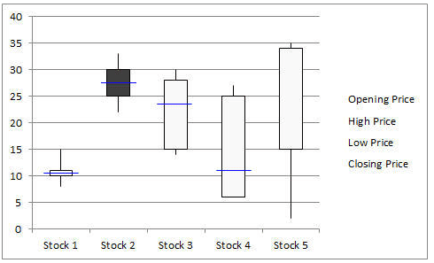
Box-and-Whisker plot, also known as a Box and Whisker plot, is a pictorial representation of continuous data. Box plots show the Max, Min, median, interquartile range Q1, Q3, and outlier data.
Run Chart
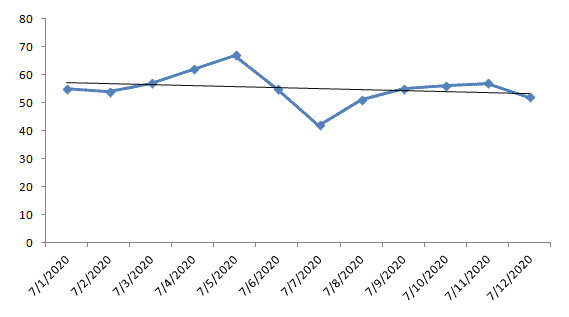
Run charts, also known as Time Series Plots, are line graphs of data plotted over time. They help to identify the pattern of the data in the time series. Run charts have no control limits, so they cannot confirm statistical control the way a control chart does. Run rules can still flag shifts, trends and other non-random patterns. However, run chart shows how the process is behaving. The advantage of the run chart is that it can signal that a special cause is present.
Scatter Diagram
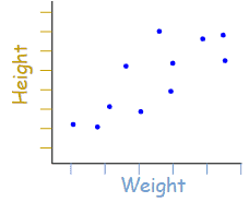
Scatter diagrams, also known as Correlation Charts or XY Graphs, plot the relationship between two continuous variables. These can include the independent variable on the x-axis and the dependent variable on the y-axis.
Histogram
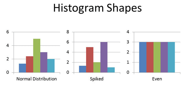
A Histogram is the graphical representation of a frequency distribution. It is in the form of a rectangle with class intervals as the base and the corresponding frequencies as the height. Particularly, there are no gaps between any two successive rectangles.
Normal Probability Plot
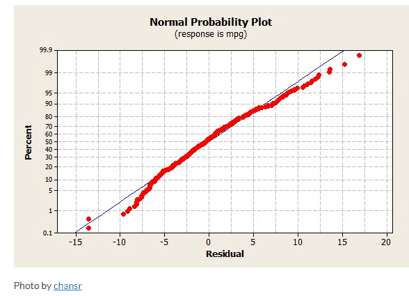
The Normal Probability Plot is a graphical method to assess whether the data set follows a normal distribution or not. This includes identifying outliers, skewness, etc. Furthermore, the Normal Probability Plot is one example of a Quantile-Quantile (Q-Q) plot.
Pareto Chart
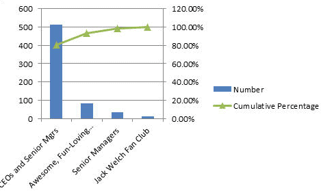
A Pareto Chart is based on the Pareto principle (the 80-20 rule). It is a combination of a bar chart and a line chart. The actual data is in descending order and uses a bar chart and cumulative data in ascending order on a line graph.
Bar Chart
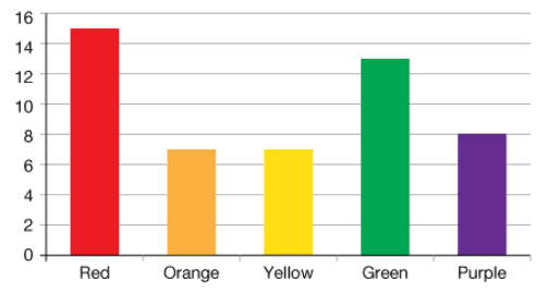
A Bar Chart displays the frequency on one axis and the values of the categorical variable on the other axis. In a bar graph, bars of uniform widths are drawn with various heights. However, the height of the bars represents the frequency of the corresponding observation.
Why Use Graphical Analysis Tools
Six Sigma teams apply a wide range of graphical tools in each phase of DMAIC.
Define
The main purpose of the Define Phase is to define the problem, identify customer requirements, and also summarize the project plan.
The project team uses various six sigma tools in the Define Phase like SIPOC (Supplier-Input-Process-Output-Customer), Process maps, value stream mapping, Project charter, SWOT analysis, and Voice of Customer.
The Six Sigma team uses graphical analysis tools. For example, they use a Bar Chart to understand a process trend, revenue loss, etc. Then, they use a Run chart to monitor customer complaints or defects over a period of time. Similarly, A Box Plot graphically represents the voice of the customer (pictorially depicts customer satisfaction with various attributes).
Measure
Measure the process performance. In fact, the main purpose of the measure phase is to collect the data that covers the project scope and also to determine what data distribution you are working with.
The project team uses various Six Sigma tools like a process flow chart, Gage R&R, Pareto Chart, and a process capability analysis in the measure phase.
Graphical tools like the Pareto Chart are used to analyze the frequency of problems and identify the majority (80%) of issues. Similarly, the Process Capability Analysis is used to assess the ability of the process to perform according to the specification.
Analyze
The main purpose of Analyze phase is to understand the root cause of the problem. Furthermore, to identify the opportunity for improvement.
Above all Six Sigma team uses most of the graphical tools in Analyze phase. Few examples like a Histogram, Scatter Diagram, Multi-Vari Chart, Time Series Chart, Normal Probability Plot, etc.
Improve
The main purpose of Improve phase is to eliminate the root causes and implement the improvements. Additionally, design the action plan to monitor the improvements.
In fact, graphical tools like statistical control charts (I-MR chart, u-chart, p-chart, and c-chart) help to monitor progress and to make necessary adjustments.
How to Pick Which Tool to Use?
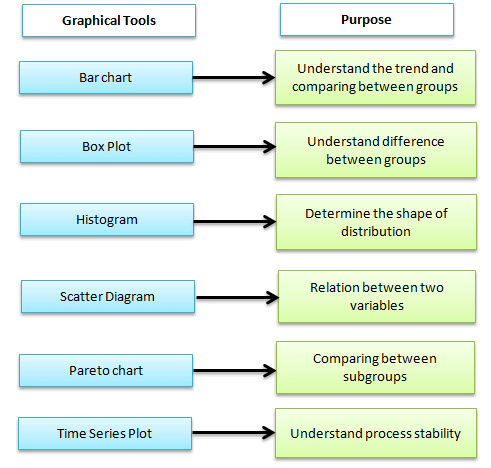
The selection of graphical tools depends on the type of data and the project’s objective. The picture below helps identify the right graphical tools based on the scenario. However, statistical analysis is required before drawing any conclusions.
How to Understand what the tools are telling you?
Often, the biggest challenge for Six Sigma teams is to understand the graph and make conclusions. In fact, it is difficult to understand the message from the graph right away. The Six Sigma team has to take time to interpret the graphs.
Each graph provides different messages like trend, frequency, dispersion, and distribution shape.
Box-and-Whisker plot is to understand the difference between the groups, outliers in the process, and maximum and minimum values. Is there any difference between the subgroup’s median?
A Histogram is used to understand the shape of the distribution. Is it symmetrical or skewed?
Scatter diagrams are to understand the relationship between two continuous variables. Is there any correlation between factors?
Time series plots are to understand the trend over time. Is the process stable over time?
Pareto Charts are to understand the frequency of the problem as well as their cumulative impact.
When you’re ready, there are a few ways I can help:
First, join 12,000+ other Six Sigma professionals by subscribing to my email newsletter. A short read every Monday to start your work week off correctly. Always free.
* * *
If you’re looking to pass your Six Sigma Yellow Belt, Green Belt or Black Belt exam, I’d recommend starting with my affordable study guide:
1)→ 🟡Pass Your Six Sigma Yellow Belt: built for ASQ, IASSC and ILSSI, 1,700+ practice questions with explanations, and six full-length mock exams for your exam
2)→ 🟢Pass Your Six Sigma Green Belt: a study guide organized by the exam Body of Knowledge, 1,300+ practice questions with detailed answer explanations, and 20 full-length mock exams
3)→ ⚫Pass Your Six Sigma Black Belt: the full Black Belt Body of Knowledge, 2,200+ practice questions with detailed answer explanations, and 20 full-length mock exams
You’ve spent so much effort learning Lean Six Sigma. Why leave passing your certification exam up to chance? This comprehensive study guide offers 1,700+ exam-like questions for Yellow Belts, 1,300+ for Green Belts and 2,200+ for Black Belts with full answer walkthroughs, access to instructors, detailed study material, and more.
Process Capability and performance (Pp, Ppk, Cp, Cpk) are specification indicators relative to process dispersion and process centering. Process capability is a statistical measurement of a process’s ability to produce parts within specified limits consistently. In other words, it is the ability of the process to meet the design specification for a service or a product.
Process capability is expressed as 6σ, where σ is the standard deviation of the process in statistical control, usually estimated from a control chart.
Process capability refers to the inherent ability of a process to produce similar parts for a sustained time under a given set of conditions. A capable process is one where almost all the measurements fall inside the specification limit. In other words, a capable process is a process whose spread on the bell-shaped curve is narrower than the tolerance range.
Why use a process capability study
Process capability study helps in product and process design, vendor sourcing, production planning, and manufacturing process control.
A few ways a process capability study helps:
Assists designers in selecting or designing processes
Establishing an interval between sampling
Specifying requirements of new equipment
Vendor selection based on process capability
Reducing variability in the manufacturing process
Short-term and long-term capability
Short-term capability is measured over a very short time period. In other words, it represents the variation at a certain time. For example, the process variation is relatively small in one shift with one piece of equipment. At the same time, long-term capability measures the variation over the duration of the entire study. If there is a shift in the process, the overall variation could exceed the subgroup variation.
In fact, short-term sigma is usually smaller than long-term sigma.
The basic interpretation is based on the underlying assumption of Six Sigma that a process will shift or drift ±1.5σ in the long term.
What are Process Capability Indices?
Cp, Pp, Cpk, and Ppk are capability and performance indicators for your process. Is a process capable? Is the process acceptable? How is the process actually behaving vs. how it theoretically could be behaving? You can ask these questions during a DMAIC project during both the Measure phase (if you have good, existing data) or the Control phase after implementing your changes.
Moreover, this article deals with an overall examination of Process Capability and performance (Pp, Ppk, Cp, Cpk).
If you’d like more depth, including calculations, etc., see these articles:
In fact, to begin to answer these questions, it all starts with customer requirements and the follow-up with what we know mathematically about the variation of the process.
Why Use Cp, Cpk, Pp, and Ppk?
Cp, Cpk, Pp, and Ppk are all parameters (indices) that can help us understand how our process operates relative to the specifications. In other words, they measure how close our process is running to its specification limits.
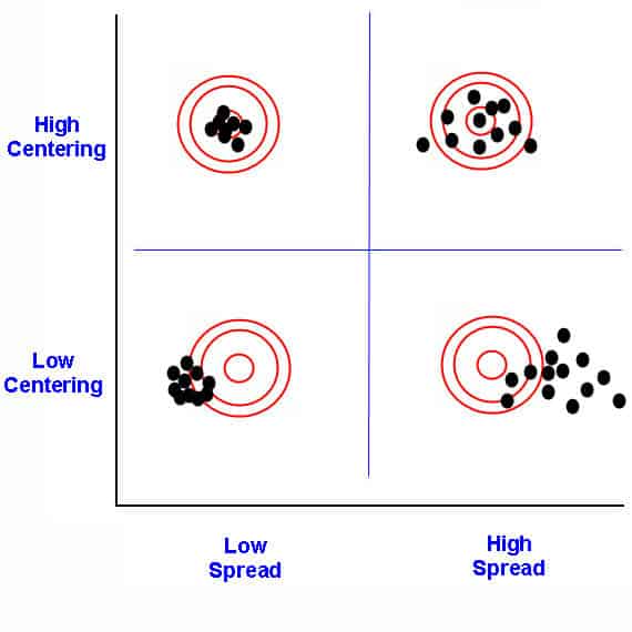
For requirements, we measure the process specifications. To determine the answers, we see how wide the process dispersion (spread of values) is and how centered the process is relative to those specifications.
The process spread vs. centering
Further on the mathematical side, we require the process to follow a normal distribution so we can take advantage of the properties there. Before using these indices to see how capable and acceptable your process is, test your process for normality. If it’s not normal, then see if you can apply a transform to get it there. If not, you may have to use non-normal distributions and methods (not part of the Six Sigma Black Belt curriculum. See the Master Black Belt guide.)
When to Use Process Capability Indices: Pp, Ppk, Cp, and Cpk
The main difference between Pp and Cp on one side and Ppk and Cpk on the other side is which standard deviation each one uses. Pp and Ppk use the overall standard deviation, calculated across all of the individual data points as one complete set, without regard to subgrouping. Cp and Cpk use the within-subgroup standard deviation, calculated from rational subgroups (pre-production runs, batches, logical sampling groups). Note that neither is a “population” standard deviation in the strict statistical sense, both are still estimated from sample data. The real distinction is overall (Pp, Ppk) versus within-subgroup (Cp, Cpk) variation, not sample versus population.
When to use Pp Ppk Cp Cpk
Differences Between Cp & Pp
The biggest difference between Cp and Pp is which standard deviation each one uses. Pp uses the overall standard deviation calculated from all of the individual data points together, without regard to subgrouping; this is why it’s suited to a new process, where you don’t yet have a stable, rational subgrouping structure. Cp uses the within-subgroup standard deviation, typically estimated using the R-bar/d2 method, which reflects only the short-term, common-cause variation of an already stable, in-control process.
Attribute & Discrete Capability
Attribute capability refers to the ability of a process to produce products or services that meet binary or yes/no criteria. Examples of attribute data include pass/fail, good/bad, or acceptable/unacceptable.
Discrete capability refers to the ability of a process to produce products or services that meet discrete or countable criteria. Examples of discrete data include the number of defects per unit, the number of calls per day, or the number of products produced per hour. Discrete capability is usually reported as defects per unit (DPU) or DPMO. Cp and Cpk need continuous data.
Both attribute and discrete capability are important for ensuring that a process meets customer requirements. The appropriate measurement technique will depend on the data type in the process.
Process Capability for Non-normal Data
In a real-time scenario, it is impossible always to fit the data into a normal distribution. If the histogram of the individual data element indicates that the data is not normally distributed, the procedure described above for determining the process capability indices does not yield the correct value for the percentage of process output exceeding the specifications.
The following are the options for better results:
Explore another known distribution that fits the data, such as exponential, lognormal, gamma, and Weibull.
Use non-linear regression to fit a curve to the data and apply numerical integration to find the area of the “tails” beyond the specification limits.
Transform the data and specification limits. The Box-Cox and Johnson transformations are the most widely used among the data transform methods. These transformations introduce a new variable that will have a more normal distribution.
Process Capability for attributes data
The control chart represents the process capability once special causes have been identified and removed from the process. A capability is defined as the average proportion or rate of non-conforming products for attribute charts.
p charts: Process capability is the process average nonconforming, p̅. Use 1- p̅ for proportion conforming to the specification.
np charts: Process capability is the process average non-conforming p̅
c charts: Process capability is the average number of nonconformities, c̅, in a sample of fixed size n.
u charts: Process capability is the average number of nonconformities per reporting unit, u̅.
The average proportion of nonconforming may be reported on a parts per million (PPM) scale by multiplying times 1,000,000.
Binomial Capability Analysis
Binomial capability analysis determines whether the percentage of defective items meets customer requirements. It is a statistical method to evaluate the ability of a process to produce products or services that meet binary or yes/no criteria. The goal of binomial capability analysis is to determine if the process can produce products or services that meet the quality requirement with high confidence.
Binomial capability analysis is used when the data is attribute data and classified as either conforming or non-conforming to a specific quality requirement. Furthermore, in binomial capability analysis, the process is characterized by a proportion, p, representing the probability that a unit will conform to the quality requirement.
Following steps to perform Binomial Capability Analysis:
Collect data on the number of conforming and non-conforming units.
Calculate the sample proportion, p̂. p̂ is the number of nonconforming (defective) units divided by the total number of units.
Calculate the standard error of the sample proportion. √( p̂ x (1- p̂) / n), where n is the sample size.
Plot the proportion defective on a p chart to check that the process is stable.
Report the percent defective with its confidence interval. You can also convert it to PPM or a process Z value.
Interpret the results to determine whether the process can confidently produce products or services that meet the quality requirement.
Preparing for a Six Sigma exam? Get the one-page Cp, Cpk, Pp, Ppk cheat sheet.
Formulas, how to judge the number, the exam rules, and a worked example on one printable page. Enter your email and I'll send it now.
You'll also get my weekly Six Sigma newsletter. Unsubscribe anytime.
Process Capability studies
A process capability study helps to identify whether a process meets customer requirements consistently over a period of time. Furthermore, a process capability study yields a prediction; hence it needs to perform the study in a controlled and stable process environment.
Concept of Stability
Process stability is one of the critical factors in process capability, as an unstable process will produce products or services that are not consistent in quality. To achieve process stability, it is important to understand the sources of variation in the process and also to take appropriate steps to control them. Furthermore, achieving and maintaining process stability is an ongoing process that requires continuous monitoring and improvement.
There are several tools and techniques exist to assess process stability and control variation, including statistical process control (SPC), control charts, and process capability analysis. These tools help to identify when a process is out of control or producing products or services outside of the desired range of variability.
Verifying Stability and Normality
If a process variation is due to a common cause, the output distribution forms a relatively stable one because the variation is constant. However, if a special cause exists in a process, the output distribution is unstable and unpredictable, leading to inaccurate results. If the variation is due to a common cause, the output will still form a distribution that is relatively stable as the variation is constant. However, if the variation is a result of a special cause, then the output is not as stable and not as predictable. In this case, a process capability study may have problems with its accuracy.
Process Capability Study Procedure
Here is the general procedure for conducting a process capability study:
Select a process to study, including process inputs, outputs, and key parameters. Use Pareto or cause-and-effect diagram-related techniques to identify the process to study.
Perform measurement systems analysis to ensure the measurement system produces accurate data.
Collect data using a sampling plan that is representative of the process. Make sure there is sufficient sample size and sampling frequency to provide a statistically valid analysis.
Select appropriate process capability analysis methods like Cp, Cpk, Pp, and Ppk.
Develop an estimate of process capability. Then, compare it with specification limits to check whether the process can meet customer requirements.
If the process does not meet the customer’s requirements, identify the root cause and initiate appropriate corrective actions to address the variation.
Validate the effectiveness of the corrective action and monitor the process periodically.
Identifying Characteristics
The selection of important characteristics is one of the crucial steps in process capability study. The characteristics should meet specific requirements such as:
The characteristics are outcomes of a process. If the Y changes, the Inputs or Xs change. Hence
Flexible to adjust the characteristics values
Able to maintain and control the influential operating parameters
Select the characteristic which significantly impacts the quality of the product or process. For example, a process may contain 20 to 30 parameters. Still, in reality, only 3 or 4 may greatly impact the process and include only those parameters in the process capability study.
Often characteristics are selected based on past history that is difficult to monitor and control.
Identifying Specifications/Tolerances
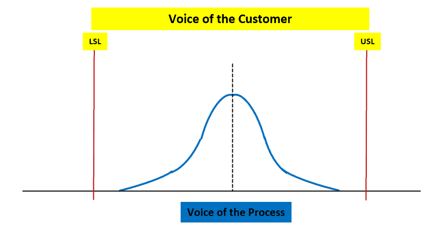
Specification limits are the boundaries set for a product or the process by customer or market performance; often, the Voice of the Customer is the input for these criteria. In other words, they mark the range of results the customer will accept.
Customers set the limit (upper and lower) on the product characteristics that define where the product works and where it does not. If the product falls outside of these limits, assume that the customer will reject the product. Specification limits are related to product design. Hence, set these limits in the design phase of the product life cycle.
Upper Specification Limit: The highest limit a customer would accept.
Example: A customer would wait in line at a drive-through for 7 minutes before being dissatisfied.
Lower Specification Limit: The lowest limit a customer would accept.
Example: A customer would expect no less than 100 M&Ms to be in a packet before being dissatisfied.
Monitoring techniques
Monitoring techniques for process capability include keeping track of the performance of a process over time to ensure that it is operating within its specified limits and producing the output that meets customer requirements. A few monitoring techniques are:
Statistical process control (SPC: Statistical Process Control (SPC) is a statistical method to measure, monitor, and control a process. It is a scientific visual method to monitor, control, and improve the process by eliminating special cause variations in a process.
Control charts: Control charts are graphical tools used to monitor a process over time. A control chart is one of the primary techniques of statistical process control (SPC). The control chart is a graphical display of quality characteristics that have been measured or computed from a sample versus the sample number or time.
Process capability indices: Process capability indices are numerical measures of the ability of a process to produce products or services within a specified range of variability. These indices can be used to monitor process performance and identify areas for improvement.
Failure mode and effects analysis (FMEA): FMEA is a technique to identify and evaluate potential failures in a process. And also to determine the potential effects of those failures on the final product or service. FMEA is a tool that helps us anticipate what might go wrong with a product or process. We can also use it to identify the possible causes and probabilities of failures.
What Can Process Capability and Process Performance Tell Us?
Process Capability Analysis tells us how well a process meets a set of specification limits based on a sample of data taken from a process. It can be used to establish a baseline for the process and measure the future state performance of the process for comparison.
Cp for processes that are under statistical control and Pp for new processes. A good analogy is parking a car in a garage. If the car is bigger than the garage, it will not fit within the specification limits and thus is incapable. This case is clear.
What about a case when our car is skinnier than the garage you’re trying to park it in (the specification width)? Can we consider our parking process a capable one? It depends on our specifications and the width of the car. Are we satisfied with the probability of 99% that we will park our car without hitting the wall? This means that one in a hundred attempts to park our car will hit the garage wall!
Different Methods to Calculate Process Capability
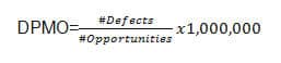
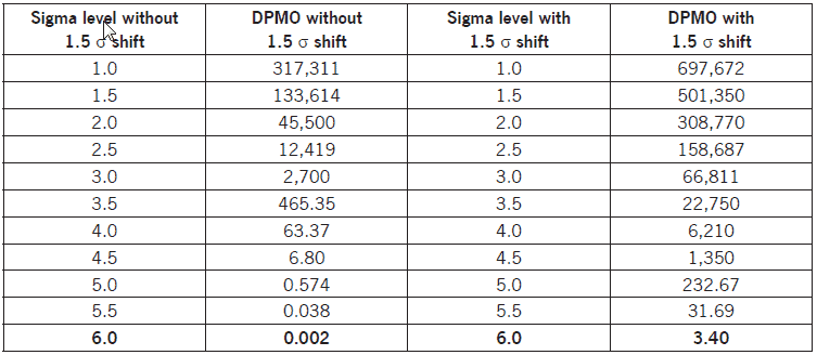
One way to calculate Process Capability is through the number of defects per opportunity. This is usually used for discrete data and in manufacturing. Usually, an acceptable number of 3.4 Defects Per Million Opportunities (DPMO).
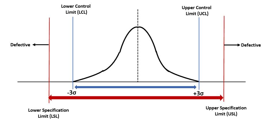
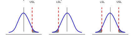
The other way to calculate Process Capability is through the use of a statistical methodology. Processes with a normal distribution of data have restrictions from one or both sides of the curve based on the Specification Limits (USL and LSL):
Shaded areas represent the probability of defects; our goal is to minimize the size of the shaded areas.
Is a Process Capable?
Process capability analysis is the act of determining if a process can meet specifications.
Here we want to use Pp for new processes or Cp for processes that are under statistical control. A good analogy is parking a car in a garage. A capable process indicates the car (process) is skinnier than the garage you’re trying to park it in (the specification width). If the car is much bigger than the garage, it is not enough to be capable of fitting within the specification limits and thus is not capable.
A capable process does not necessarily mean it is acceptable. Using the garage example, the car may have crashed into the side or may have missed it completely. This point reflects how centered a process is. We can measure this using Ppk or Cpk.
A Note on a Process Being Both Capable and Acceptable
A process is said to be capable and acceptable when it meets customer requirements. Specifically, having zero defects is usually unrealistic and not usually a part of customer requirements. A process could be capable but unacceptable because it is poorly centered and ends up outside the spec limits. For example, a car could fit in the garage, but the process of parking it could have it just as easily end up driving through your front door as it could safely parked!
Six Sigma Process Capability & Performance Limits
According to Six Sigma philosophy, Cp or Pp should be at least 2.0, and Cpk or Ppk at least 1.5. Six Sigma deems a process acceptable only after achieving a maximum defect rate of 3.4 ppm opportunities. Furthermore, there is a direct correlation between Cpk or Ppk and parts per million defects. Only processes that meet both thresholds achieve this goal (3.4 defects per million).
Control Limits, Specification Limits, and Process Capability
Keeping a process in control limits is not sufficient to achieve good quality. Quality is always dictated by the user. For that we use specification limits when assessing process capability. The process specifications used in process capability are the voice of the customer and control limits of Statistical Process Control are the voice of the process.
It is very possible to have great process control (indicated on a control chart) yet have poor process capability. That would be a mismatch of where the process is centered versus where the customer wants it to be centered. Either that or the process has more variability than the customer desires.
Cp vs. Cpk
Cp and Cpk both use the same within-subgroup standard deviation, and both apply to a process that’s already under statistical control; the difference between them is centering. Cp only measures whether the spread of the process fits inside the specification limits; it says nothing about whether the process is actually centered between those limits. Cpk measures that same spread, but relative to whichever specification limit the process mean is closest to, so it accounts for centering. Cp is always greater than or equal to Cpk; the two are equal only when the process is perfectly centered.
Pp vs. Ppk
Pp and Ppk both use the same overall standard deviation, calculated from all of the individual data points, and both are used before you’ve confirmed the process is under statistical control; the difference between them, again, is centering. Pp only measures whether the overall spread of the process fits inside the specification limits. Ppk measures that same spread relative to whichever specification limit the process mean sits closest to, so it accounts for centering. As with Cp and Cpk, Pp is always greater than or equal to Ppk, and they’re equal only when the process is perfectly centered.
Pp vs. Cp (Capability Indices)
In fact, both Cp and Pp monitor indices for the spread of your process compared to the specification spread. However, use Cp when a process is under statistical control and Pp when a process is initially starting out.
Uses for Cp & Pp
Used to see if a process is capable.
Neither is concerned with centering. Cp or Pp takes into account dispersion, NOT centering. Since Cp does not consider process centering, it cannot be used to determine whether a process is acceptable.
Cpk & Ppk both take centering into account, so use them to see if a process is acceptable.
In addition, both Cp & Pp are NOT concerned with the control of a process. The term “control” infers an element of time, and Cp or Pp is merely a snapshot of the process variation at a given point in time.
For example, a Cp of < 1 does NOT indicate a process is out of control. “Control” is controlling variation over a period of time. A Cp is a snapshot at a point in time but does not indicate that the process is in control.
If Cp or Pp >1, Tolerance is > spread; the Process has the potential to be capable (depending on centering).
A CP of >1 doesn’t mean quality. One could have a Cp of 400 and produce 100% defects because the process was not centered within the specification limits.
If Cp or Pp <1 process spread is > tolerance, the variation will never fit, and the process will never be capable.
A Cp of < 1 does NOT indicate a process is out of control. “Control” is controlling variation over a period of time.
If 0< CP <1, then the specifications are that percentage of the process.
Ex. Cp 0.70 = 70%. A Cp of 0.70 means the specifications are 70% of the process.
Ppk vs. Cpk (Acceptable Performance)
Cpk and Ppk both account for how centered a process is relative to the specification limits, not just how wide its spread is. The difference between them is the same as the difference between Cp and Pp: Cpk uses the within-subgroup standard deviation and applies to a process already under statistical control, while Ppk uses the overall standard deviation and applies to a new or not-yet-stable process. In practice, this gives you a useful diagnostic: once a process is stable, Cpk and Ppk converge toward nearly the same value, since the within-subgroup and overall standard deviations become close. If the two numbers stay far apart even after the process has been running a while, that itself is a sign the process still isn’t in statistical control.
Uses for Cpk & Ppk: Is The Process Acceptable?
Cpk or Ppk considers centering, and thus it helps to determine if a process is acceptable.
Ways to measure the capability of a process.
Reflect on the actual performance of the process.
Both Cpk and Ppk can be negative numbers. So, it means that, on average, the process is not meeting customer requirements.
Can Cpk or Ppk be Negative? What does a negative Cpk or Ppk Indicate?
Yes, it is possible for Cpk and Ppk to be negative. Let’s look at the equation. For simplicity, we will use the Ppk.
Ppk = [ USL – x(bar) ] / 3 s
Moreover, it is impossible to have a standard deviation be negative, so that would mean that x(bar) was larger than the Specification Limit. In other words, the process average is out of specification.
This could indicate that the process mean has drifted over either the upper specification or the lower one. This is not good because it means that the process is not meeting customer requirements.
Pp, Ppk vs. Cp, CPK
Cp & Cpk use an estimate for the standard deviation using the R Bar / d2 method.
Pp and Ppk are usually the more conservative pair, because overall s is usually larger than within-subgroup sigma.
Use Pp & Ppk when you are initially setting up your process.
Use Cp & Cpk once the process is in a state of statistical control.
Cpk is less than or equal to Cp, and Ppk is less than or equal to Pp.
Interesting video on assessing Ppk and Cpk in Minitab.
When you’re ready, there are a few ways I can help:
First, join 12,000+ other Six Sigma professionals by subscribing to my email newsletter. A short read every Monday to start your work week off correctly. Always free.
* * *
If you’re looking to pass your Six Sigma Yellow Belt, Green Belt or Black Belt exam, I’d recommend starting with my affordable study guide:
1)→ 🟡Pass Your Six Sigma Yellow Belt: built for ASQ, IASSC and ILSSI, 1,700+ practice questions with explanations, and six full-length mock exams for your exam
2)→ 🟢Pass Your Six Sigma Green Belt: a study guide organized by the exam Body of Knowledge, 1,300+ practice questions with detailed answer explanations, and 20 full-length mock exams
3)→ ⚫Pass Your Six Sigma Black Belt: the full Black Belt Body of Knowledge, 2,200+ practice questions with detailed answer explanations, and 20 full-length mock exams
You’ve spent so much effort learning Lean Six Sigma. Why leave passing your certification exam up to chance? This comprehensive study guide offers 1,700+ exam-like questions for Yellow Belts, 1,300+ for Green Belts and 2,200+ for Black Belts with full answer walkthroughs, access to instructors, detailed study material, and more.
The main objective of a lean system is to augment the effectiveness and efficiency of various processes in the organization by reducing waste in operations like long lead times, defects, and bottlenecks in material and information flow. One tool that can be used is ‘Value Stream Mapping.’
Value stream mapping visually represents the organization’s flow of materials and information. It helps to identify, demonstrate, and reduce waste and creates effective flow through all the processes in the manufacturing organization.
A value stream map shows all the value-added and non-value-added activities needed to make the product. It consists of the process flows starting from the raw materials to making the product finally available in the hands of the customers.
What Does Value Stream Mapping Do?
Graphically illustrate the flows of materials and information in a process. It displays the interaction between multiple organizational functions: manufacturing and ancillary functions.
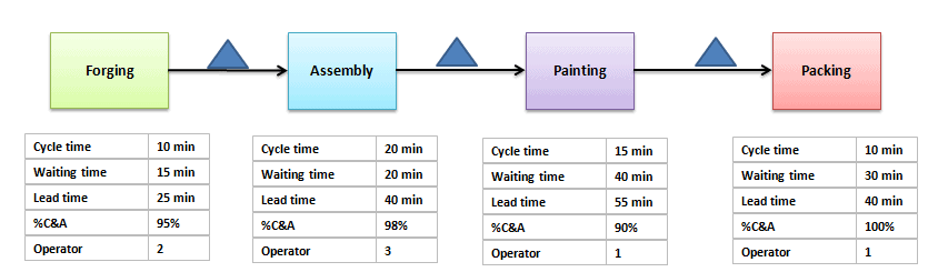
Pinpoint the problem areas, inefficiencies, defects, and bottlenecks more efficiently as it integrates and maps the information and material flow along with the sequence of tasks. It even shows the cycle times and lag times between different tasks.
Involves all the stakeholders in each stage of the process; hence, it becomes easy to develop and implement countermeasures to facilitate organizational cultural change. It provides a proper presentation of all the limiting factors.
Continuous improvement is facilitated since the direction can be focused on lean transformation teams, front-line supervision, and upper management.
The first step is to select the product or product family, decide on the improvement goal and train the team for value stream mapping. Select a cross-functional team and include all the stakeholders of the process. Then, walk through the physical path of the material or information flow. It is necessary to map all the primary as well as secondary flows.
While walking through all the material flow paths, observe and document all the communication points carefully. This will help to prepare the current state value stream map.
Identify the start and endpoints of your process.
In the end, your process owner or project sponsor is the final rule on when a process begins and ends, but in a value stream analysis, this is typically from the moment a customer requests to the moment they receive the product. Arguments could be made for capturing the whole process by including things like transaction settlement (funds clear an account, restocking or retooling takes place, all “technical debt” is completed, etc.)
Draw the process flow.
Map your process, including sub-steps. It’s helpful to trace the flow of one unit (product or service) going through the process.
Note areas that require inputs or outputs. Does that alter your diagram? Did you miss a step? Be sure to include those interactions with external teams.
Include metrics for each process step.
What measures you take depends on what kind of project you are doing. What can you afford to measure? Some processes are trickier or more expensive to measure than others. Even with unlimited resources, the spread and center of your process distribution might affect the measures you need. Perhaps an average is OK in a normal distribution case, but you might want to measure the median in another.
Before measuring, you may want to validate your measuring systems first / auditors to ensure their accuracy with a repeatability and reproducibility study. Gathering this data can be time-consuming; it is best to get it right to the precision required the first time. No matter what you measure, you might want to test your measurement tools.
What are the bounds of the case? The lower bound (or fastest time) might be the ‘happy path.’ The upper bound (or slowest time) might be the worst-case scenario.
What is the average time, or most likely time?
What is the median time?
Is there any changeover or prep time required?
What’s the uptime?
What are the resources in each step?
Manpower: how many people, how many shifts?
What are the machine’s capabilities?
What is the throughput of this step and delivery performance?
How much inventory stacks up?
Step 2: Value Stream Mapping
In this step, analyze the current state value stream map with all the stakeholders to gain consensus on the current performance of the process. Next, identify the current process’s limiting factors, deficiencies, defects, and bottlenecks. The performance and cost of each limiting factor should be quantified.
It is also important to identify the root causes and not the symptoms of the limitations of the current state value stream map. Based on the root causes of the limitations, cost-effective solutions should be developed. Finally, the current state value stream map should be amended to reflect the proposed solutions and changes to remove the limitations of the process. The amended value stream map is now called the ‘future state value stream map.’
Look at the value being delivered and the waste incurred.
Note any wastes, including, but not limited to, wait time, rework time, retooling, and downtime.
Cycle time is how often a process step completes one unit, timed by watching the step. Lead time is the time one unit takes to move through the whole process, waits included.
Touch time is the total time someone is physically working on the unit. It is not the same as cycle time. It is also different than the overall time it takes to complete a process step or task in a stream from start to finish because the waste is not built in.
This is heavily dependent upon defining your starting point and your endpoints. A SIPOC can help you identify these. In the end, the process owner (or the project sponsor) has the final rule on when a process begins and ends.
Sales: An example lead time starts when a prospect first contacts your company and ends when they complete a purchase.
Hospital: An example could be from when the patient enters the ER to when they are discharged.
Step 3: Improve
How can we cut out, remove, or avoid those wastes we identified? What are the bottlenecks in our process? What step in the process stream has the slowest throughput or cycle time? Is there a way to make that more efficient?
Before implementing the future state value stream map, socialize and gain consensus from all stakeholders. Then, the changes need to be implemented, and in that process, the affected procedures, bills of materials, and training materials should be modified. Training should be imparted to the staff based on the new procedures and requirements. Finally, implementing the changes should be facilitated on a descending priority basis.
Optimize the Whole.
The point isn’t to achieve a high score for any individual process step but rather to complete a service or produce a product for a customer quicker, utilizing fewer resources while maintaining excellent quality.
Step 4: Sustain
The implemented changes should be verified and validated by establishing and measuring performance and cost-related parameters using effective key performance indicators. The new standard procedures should be monitored and reinforced continuously.
Example: Building a Value Stream Map
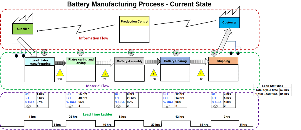
Value Stream Mapping (VSM) is used in lean management and continuous improvement methodologies to visualize and optimize processes within an organization. Here’s a worked example of building a current-state map.
Example: XYZ is a battery manufacturing company. These batteries are sent to the distribution agency (customer) based on their demand. XYZ produces the batteries, involving lead plates process, curing & drying of plates, assembly, battery charging, and finally, shipping the batteries to the distribution agency on a daily basis. Lead coils and other components are supplied by ABC supplier twice a week.
XYZ operates for 22 days a month with 2 daily shifts of 8 hours each. It receives orders from the distribution agency on a quarterly and monthly forecast basis. XYZ releases the Material Requirement Plan (MRP) to the plant and the supplier on a weekly basis, based on inventory and customer demand. Additionally, they share the daily schedule with the shipping department.
Once you have a current-state map like this one, the next step is Value Stream Analysis: critically examining the map to find bottlenecks, wait times, and waste, and turning what you find into specific improvements. See the full Value Stream Analysis guide for how that’s done, including a continuation of this same battery manufacturing example through to its future-state results.
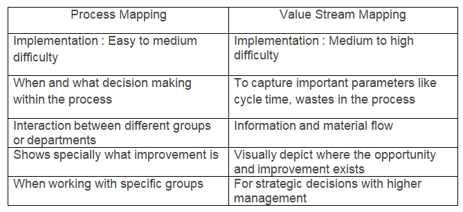
Difference between Process mapping and Value stream mapping (VSM)
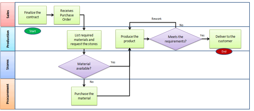
Process mapping is a tool that graphically shows a process’s inputs, actions, and outputs in a clear, step-by-step map of the process. Process mapping specifies the tasks within the function and also shows the interaction between functions or departments. It helps to visualize the process’s details closely and guides decision-making.
Value stream mapping visually represents the organization’s flow of materials and information. It shows important parameters like cycle time, lead time, inventory or waiting time, percent complete, and the number of operators. It helps identify, demonstrate, reduce waste, and create effective flow through all manufacturing or business processes. Three important steps of VSM:
Create an as-is current state process of how an organization delivers products and services to the customers.
Identify wastes in the process and draw the proposed improved state map using lean principles.
Develop action plans to achieve the proposed improved future state.
Organizations select either process mapping or value stream mapping based on business requirements. Use VSM to determine how much time the product spends on each step and waste in the process. At the same time, process mapping shows a series of steps and determines the decision-making within the process.
Value Stream Videos
A great introduction from Gemba Academy
A great practical example from Gemba Academy
ASQ Six Sigma Green Belt Value Stream Questions
Question: In order for value flow analysis to be effective, a team must take which of the following steps first?
(A) Define the value stream (B) Eliminate backlogs in the value stream (C) Identify overlapping functions in the value stream (D) Identify specific work practices within the value stream
Answer:
A: Define the value stream. This includes a starting point and an ending point of the process. You cannot do any of the other answers until you have mapped the value stream.
[/membership]
When you’re ready, there are a few ways I can help:
First, join 12,000+ other Six Sigma professionals by subscribing to my email newsletter. A short read every Monday to start your work week off correctly. Always free.
* * *
If you’re looking to pass your Six Sigma Yellow Belt, Green Belt or Black Belt exam, I’d recommend starting with my affordable study guide:
1)→ 🟡Pass Your Six Sigma Yellow Belt: built for ASQ, IASSC and ILSSI, 1,700+ practice questions with explanations, and six full-length mock exams for your exam
2)→ 🟢Pass Your Six Sigma Green Belt: a study guide organized by the exam Body of Knowledge, 1,300+ practice questions with detailed answer explanations, and 20 full-length mock exams
3)→ ⚫Pass Your Six Sigma Black Belt: the full Black Belt Body of Knowledge, 2,200+ practice questions with detailed answer explanations, and 20 full-length mock exams
You’ve spent so much effort learning Lean Six Sigma. Why leave passing your certification exam up to chance? This comprehensive study guide offers 1,700+ exam-like questions for Yellow Belts, 1,300+ for Green Belts and 2,200+ for Black Belts with full answer walkthroughs, access to instructors, detailed study material, and more.
When we use a sample group to gain insight into an entire population, whether we’re talking about people or a product built in a factory, we risk the sample group not completely reflecting the whole population. Therefore, we need confidence intervals.
Further, we use confidence intervals to calculate a degree of certainty that the sample group accurately represents the entire population from which they were drawn. Another way of thinking of it: if you drew a same-sized sample hundreds of times and built an interval from each one, a set percentage of those intervals would contain the population mean. That percentage is the confidence level.
A confidence interval is a range of values built from one sample. It gives a plausible range for the population mean, at a stated confidence level.
This page covers every kind of confidence interval you’ll need for your exam. Jump straight to the one you need:
New to the concept of estimating a population from a sample? Start with Point and Interval Estimation first, then come back here for the worked examples of each type.
Confidence Interval vs. Confidence Level
A confidence interval is a range of values that probably contain the population mean.
A confidence level is the percentage of intervals that would contain the population mean if you repeated the sampling many times. It equals 1 – α. A 95% level means about 95 of every 100 intervals built this way capture the true mean.
Confidence Interval vs. Prediction Interval
A prediction interval gives the range where the next single data point will probably fall. They tell you about the distribution of data values, whereas confidence intervals tell you about a probable population mean.
Estimating Population Mean and Standard Deviation
In most cases, we won’t know the mean and standard deviation for an entire population. However, we can calculate the mean and standard deviation for each of our samples. So we can use the sample figures to estimate those of the whole population. This is what we call a point estimate.
Once we find the point estimate, we also need to know how accurate it is. The Central Limit Theorem helps here. With a large enough sample (30 or more is the usual rule of thumb), the sample mean follows an approximately normal distribution. That distribution centers on the population mean. Its standard deviation, called the standard error, is σ/√n. That is what lets us put a margin of error around a sample mean.
Margin of Error
The margin of error is the maximum expected difference between the actual population parameter and a sample estimate of the parameter. In other words, it is the range of values above and below the sample statistic.
Surveys use the margin of error widely. It tells you how much uncertainty the results carry.
Margin of error ≈ 1/√n (a quick rule of thumb for a 95% interval on a proportion near 50%; the exact formula is below)
Where n= sample size
The margin of error is the critical value times the standard error. For the same sample size and spread, a higher confidence level needs a bigger critical value, so the margin of error grows. A bigger sample shrinks the standard error, so the margin of error shrinks.
For example, to estimate the confidence interval, we may use X̅±E
E is the margin of error.
Confidence interval = X̅±Zα/2*σ/√n (use this when the population standard deviation σ is known)
Where σ = population standard deviation
Zα/2 = normal distribution value for the desired confidence level
n = sample size
X̅ = sample mean
When σ is unknown and you only have the sample standard deviation s, swap Z for t with n – 1 degrees of freedom: X̅±tα/2*s/√n. Sample size does not decide between Z and t. Knowing σ does.
Z Scores
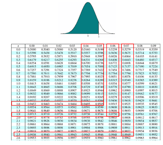
This page uses a cumulative z table: each value is the area to the left of z, so a 95% confidence level (0.025 in each tail) means finding 0.975 in the table, which gives 1.96. If your handbook’s table shows the area from the mean (0 to z), look for 0.475 instead; if it shows the upper tail, look for 0.025.
A Z score is the number of standard deviations between a data point and its mean. Thus, you can use a Z-score table to find the corresponding Z-score for common confidence levels or calculate the α value using this formula:
α = 1 - confidence level
If your desired confidence level is 95%, then your calculation would look like this:
Common confidence levels and corresponding Z scores
Confidence Level
Z Score
90%
1.645
95%
1.96
99%
2.576
Confidence Interval Question Using Z-Score
Question: We conduct a random survey of 500 newly-enrolled university students. We know that the standard deviation for university enrollment age is eight years. The mean age of our sample is 24. Calculate the confidence interval for all first-year university students with a 99% confidence level to 3 decimal places.
Calculation: We know the population standard deviation σ, so use a Z-score. A 99% confidence level requires a Z-score of 2.576.
Zα/2 = 2.576, X̅ = 24, σ = 8 and n = 500
Margin of error E = Zα/2*σ/√n = 2.576*8/√500 = 0.922
Confidence interval = X̅±Zα/2*σ/√n = 24±0.922
Answer: Hence, the confidence interval for the age of first-year university students is 23.078 to 24.922, with a 99% confidence level.
Confidence Interval Question Using T-Score
Question: A factory produces tennis balls. A sample of 19 balls is taken from one factory production day. The mean weight of the sample balls is 58.2g. The standard deviation for the sample balls is 0.4g. Calculate the confidence interval with a confidence level of 95%.
Calculation: The population standard deviation is unknown. All we have is the sample standard deviation s, so use a T-score, which uses a t-distribution. Sample size does not decide between Z and t. Knowing σ does. Finding a confidence interval for a mean is a two-tailed interval.
You’ll need the alpha value. To calculate it, use this simple equation:
You also need the degrees of freedom (df), which is the sample size minus one. Or in equation form:
df = n - 1
df for this question is 18.
So, use a T-table to look up the t-score for a two-tailed interval with an α of 5% (0.025 in each tail) and a df of 18: the answer is 2.101.
tα/2=2.101, X̅=58.2, s=0.4 and n=19
Margin of error E = tα/2*s/√n = 2.101*0.4/√19 = 0.193
Confidence interval = X̅±tα/2*s/√n = 58.2±0.193
Answer: Hence, a 95% confidence interval for tennis balls produced in the factory is 58.007 to 58.393 g.
Calculating the Confidence Interval Comparing Two Population Means
Using samples from each population, you can also use confidence intervals to compare two population means. Use this method to compare two manufacturing methods, or to look for a difference between two groups of people (for example, smokers and nonsmokers).
The confidence interval for comparing two means is a range of values in which the difference between those two means probably lies. If the interval includes 0, the data do not show a real difference. If the whole interval sits above or below 0, they do.
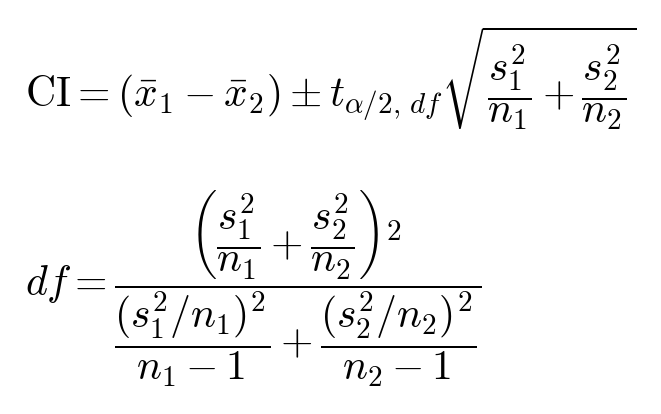
We almost never know the population standard deviations. We only have the sample standard deviations, s1 and s2. So use a t interval, not Z.
Default: unequal variances (Welch’s t interval). Use this unless the question tells you to assume equal variances.
High blood pressure has been causally linked to smoking tobacco products. To test this, you want to compare systolic blood pressure between smokers and nonsmokers. You’ll use a confidence level of 95%.
You have 45 smokers and 56 nonsmokers. The two groups are made up of comparable people (similar age, gender and health). That makes the comparison fair. It is not the same as assuming equal variances.
In the sample group of smokers, the mean systolic rate is 138.
In the sample group of nonsmokers, the mean systolic rate is 135.
The sample standard deviation for smokers is 16.5.
The sample standard deviation for nonsmokers is 14.9.
These are sample standard deviations (s), not population values (σ). So use t, not Z.
Answer: With 95% confidence, the true difference in mean systolic pressure (smokers minus nonsmokers) is between -3.29 and 9.29 (Welch). The pooled version gives -3.21 to 9.21. Both intervals include 0. So these samples do not show a real difference in systolic pressure between smokers and nonsmokers at the 95% level.
The margin of error is the half-width of the interval: 6.29 for Welch, 6.21 for pooled. We are 95% confident the true difference lies within that distance of the sample difference of 3. With samples this large, a Z of 1.96 gives almost the same answer (±6.20). On the exam, use t whenever you only have s.
Additional Confidence Intervals Videos
Confidence intervals for Variation
The point estimate for σ is s. s2 is an unbiased estimate of σ2.
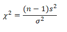
Use the chi-square distribution to construct a confidence interval for the variance and standard deviation.
If the random variable x has the normal distribution, then this statistic follows a chi-square distribution with n – 1 degrees of freedom:
For sample size n > 1
Confidence intervals for variation:
Where n= sample size
s2 = point estimate of variance (the sample variance)
Example: XYZ pharmaceutical company randomly selected 25 samples of flu medicines. The sample variance is 6 mg2. Assume the weights are normally distributed and construct a 99% confidence interval for the population variance.
n=25
Degrees of freedom = n -1 = 24
s2 = 6
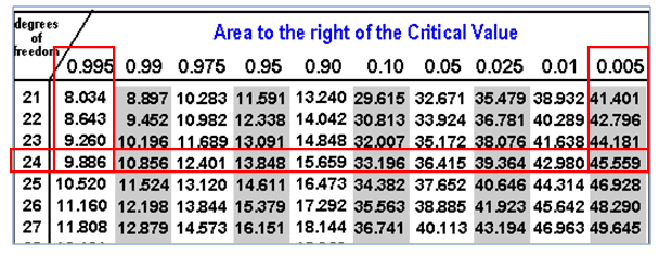
χ2α/2 = 45.559 (area of 0.005 to the right, 24 df)
χ21-α/2 = 9.886 (area of 0.995 to the right, 24 df)
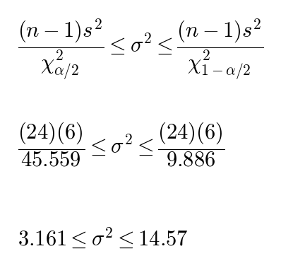
Confidence intervals for variation:
Hence, with 99% confidence, you can say that the population variance is between 3.161 and 14.57 mg2. Take the square root of each end for the standard deviation: 1.778 to 3.817 mg.
Confidence intervals for Proportion
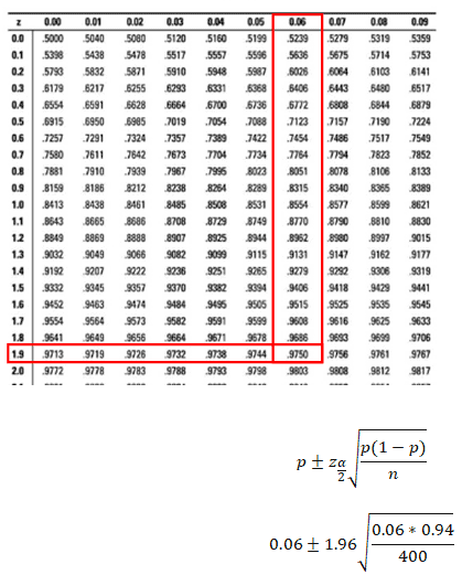
The Central Limit Theorem says that with large samples, the sample proportion follows an approximately normal distribution. When np and n(1 – p) are both at least 5, you can use the normal (Z) distribution to build a confidence interval for a proportion.
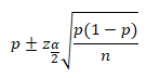
The confidence interval for a proportion is:
Where:
n=sample size
p = sample proportion (your estimate of the population proportion)
Zα/2 = Z value for your confidence level, from the Z table
Example: In a bulb manufacturing unit, 24 defective bulbs were identified in a sample size of 400 bulbs. Calculate the 95% confidence interval for the proportion.
n=400
p = 24/400 = 0.06
1-p = 0.94
Check: np = 24 and n(1-p) = 376. Both are at least 5, so Z is fine.
Zα/2 = 1.96 (95% confidence)
0.06±0.0233
0.037≤p≤0.083
So, with 95% confidence, the population proportion is between 0.037 and 0.083.
What is the Difference Between Control Limits and Confidence Intervals?
Control limits come from your process data. They usually sit at the average plus or minus 3 standard deviations of the plotted statistic. They show what the process actually does. A process that stays inside its control limits with no unusual patterns is stable, or in statistical control.
These are different from Specification limits. Specification limits come from the customer or the business. They say what is acceptable. They do not belong on a control chart. A colleague once described them as if the process goes above this level, we all must update our resumes. So, if it goes below this other limit, don’t worry about updating resumes; no one will ever hire us again!
Confidence Interval
Confidence intervals are a device of statistics for when you do not have perfect knowledge of all of the data. For example, imagine you are trying to infer the chance of some event happening by sampling from a population. Let’s take US voting polls. CNN can’t possibly get all of the voting data, but they can sample the population through exit polls. From that sample, they can predict the winner. So, the question is, how sure and certain are they of how accurate their answer is? Are they 90% certain? Are they 95% certain? 99.5%? It all depends on the confidence level required. Thus, you get answers like, “Candidate X has 52% of the vote, plus or minus 3 points, at a 95% confidence level.”
The confidence level is how sure you are that your interval captures the true population value. The confidence interval is that range. Neither one is a control limit. Control limits describe how a process behaves over time.
When you’re ready, there are a few ways I can help:
First, join 12,000+ other Six Sigma professionals by subscribing to my email newsletter. A short read every Monday to start your work week off correctly. Always free.
* * *
If you’re looking to pass your Six Sigma Yellow Belt, Green Belt or Black Belt exam, I’d recommend starting with my affordable study guide:
1)→ 🟡Pass Your Six Sigma Yellow Belt: built for ASQ, IASSC and ILSSI, 1,700+ practice questions with explanations, and six full-length mock exams for your exam
2)→ 🟢Pass Your Six Sigma Green Belt: a study guide organized by the exam Body of Knowledge, 1,300+ practice questions with detailed answer explanations, and 20 full-length mock exams
3)→ ⚫Pass Your Six Sigma Black Belt: the full Black Belt Body of Knowledge, 2,200+ practice questions with detailed answer explanations, and 20 full-length mock exams
You’ve spent so much effort learning Lean Six Sigma. Why leave passing your certification exam up to chance? This comprehensive study guide offers 1,700+ exam-like questions for Yellow Belts, 1,300+ for Green Belts and 2,200+ for Black Belts with full answer walkthroughs, access to instructors, detailed study material, and more.