
Analyze Phase (DMAIC)

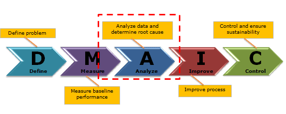
Analyze phase is the third phase of DMAIC. The main activity in the Analyze phase is to identify the potential root cause of the problem and arrive at the actual root cause. In other words, let’s use the data obtained in the Measure Phase to identify the root causes that we want to fix. One of the key activities here is process characterization: identifying and quantifying the significant sources of variation in the process.

During the measure phase of DMAIC, the project team should clearly understand the problem statement. Six sigma teams use various statistical tools in the Analyze phase to identify the root cause(s).

Six Sigma Phases

Six Sigma is a systematic problem-solving approach that is centered around defect elimination and variation reduction. This leads to process improvement.

One of the principal tools in Six Sigma is using the DMAIC methodology. (Also see DMAIC Overview). Particularly, DMAIC is a logical framework that helps you think through and plan improvements to a process to achieve a Six Sigma level of excellence.

There are five phases that are used in the DMAIC method.
Analyze Phase (DMAIC)

During the Analyze phase, use the data-driven approach to identify the problem’s root cause(s). Often, teams conclude the root cause without proper analysis; hence, the Analyze phase is critical in DMAIC. At the end of this phase, the six sigma team identifies the most significant impact on CTQs.

Analyze Phase of DMAIC Goals

  • Use measure data to identify the probable causes of the problem
  • Identify the actual root cause using brainstorming, 5 why, and other techniques
  • Find the critical root cause that has the highest impact on CTQ
  • Verify the root causes using appropriate statistical tools and techniques like hypothesis testing

Analyze Phase of DMAIC Overview

The Analyze phase is approximately 2 to 3 weeks process based on the project inputs. In particular, all the relevant stakeholders’ involvement is key in identifying the root causes.

The Analyze phase is all about reviewing the process map to improve efficiency, listing the probable root causes, and identifying important factors/inputs that greatly impact the output using statistical tools like hypothesis testing. Multiple tools and concepts are available in the Analyze phase of Six Sigma.

Process map Analysis (Identify Value and non Value activities)

Detailed Process Map: A process map is a tool that graphically shows the inputs, actions, and also outputs of a process in a clear, step-by-step map of the process. 

The process map illustrates the relationship between inputs (X) and outputs (Y). Create a process map of all the activities required to convert raw materials into output (Y) and then identify the critical to quality (CTQs) factors in the process.

Value Stream Mapping: Value stream mapping visually represents the flow of materials and information throughout the organization. Value stream mapping constitutes all the value-added as well as non-added values required to make the product. It consists of the process flows starting from the raw materials to making the product finally available in the hands of the customers.

Waste Analysis

Classic Wastes are looked at as a blockage against productivity. It is not possible to enhance the top line in a highly competitive world by increasing the prices. Hence, it is necessary to build effective systems, and one of the ways is to understand the ‘wastages’ and eliminate them. Following are the seven classical wastes in an organization.

  • Overproduction: This wastage occurs when the production output is much more than the requirement of the next process or customer. 
  • Inventory: Inefficient planning of inventory and ordering either less or more of inventory further leads to wastage. 
  • Waiting: Wastage of the operator time in avoidable events like failure of equipment, late arrival of necessary tools, lack of trained staff, inefficient planning, and idle machine time leads to wastage. 
  • Motion: Wastage due to unnecessary movement of parts and products between different processes and places. 
  • Defects: Defects and broken parts add to customer dissatisfaction, and the company would be busy solving problems, reworking, and even paying off to the customers for the defects.
  • Over-processing: Unnecessary performance of any process due to design failure or usage of poor quality tools and processes.
  • Transport & Handling: This Muda can be observed in many activities, like shipping damage and packing material wastage.

List Potential Causes

The focus of analyze phase is to identify the possible root causes of the problem.

Root Cause Analysis: Root cause analysis is a collection of tools and processes we can use to determine the most important causes for an issue we are trying to resolve.

Organize the potential causes to show relationships

  • Brainstorm: Brainstorming is a method for generating a large number of creative ideas in a short period of time. 
  • 5 Whys:  It is a simple tool to ask “Why” until we can’t ask “Why” again. 5 is a good rule of thumb (of course arbitrary). By often querying “Why”, we can quickly reach the underlying causes of a problem.
  • Fishbone Diagram:  It is a pictorial diagram showing possible causes (process inputs) for a given effect (process outputs). In other words, it is a visual representation to find out the cause(s) of a specific problem.
  • Fault Tree Diagram: Fault tree analysis (FTA) is a graphical tool to explore the causes of system-level failures. It uses boolean logic to combine a series of lower-level events. It is basically a top-down approach to identify the component level failures (basic event) that cause the system level failure (top event).
  • Affinity Diagram: An affinity diagram is a good technique for identifying & displaying potential root causes for unfamiliar problems.
  • Tree Diagram: A Tree diagram helps you break down big concepts into progressively greater detail. The idea here is to systematically break down a concept into its constituent pieces.        
  • Interrelationship Diagram: An interrelationship digraph (aka network diagram) helps you see relations and influences between several concepts. You can also use it to identify critical issues and key drivers of a problem.
  • FMEA: Failure Mode Effects Analysis (FMEA) is a tool that helps us anticipate what might go wrong with a product or process.

Prioritize final list

Put the diagram of the current process steps, defined outputs & the factors influencing those outputs, and a table listing the process analysis results. Include all data sources used, how data was collected, and the tools used in analyzing the data (hypothesis testing). Use this to prioritize the final Potential Cause list.

Data Analysis & Identify the Root Cause

After the six sigma team identifies the Potential Cause list, it is required to determine its true root cause. This is where we use various methods and mathematical tools to verify our assumptions. We can also use advanced techniques to compare data against each other and even to make predictions.

Mathematical Tools

Central Limit Theorem: The Central Limit Theorem states that the distribution of the sample means approaches normal regardless of the shape of the parent population.

Distribution Types: Data distribution is a function that specifies all possible values for a variable. It also quantifies the relative frequency (probability of how often they occur). It’s important to determine the kind of distribution of that population. It helps to choose the correct statistical methods when analyzing it.

Continuous distribution

A continuous distribution containing infinite (variable) data points that may be displayed on a continuous measurement scale. 

  • Normal Probability: It is a symmetrical bell shape curve with higher frequency (probability density) around the central value. The frequency sharply decreases as values are away from the central value on either side.
  • Lognormal Distribution: A continuous random variable x follows a lognormal distribution if its natural logarithm, ln(x) follows a normal distribution.
  • F Distribution: The F distribution extensively use to test for equality of variances between two normal populations
  • Chi-Square: The chi-square distribution results when independent variables with standard normal distribution are squared and summed.

Discrete Distributions

A discrete distribution resulting from countable data that has a finite number of possible values. Furthermore, discrete distributions can be reported in tables, and the respective values of the random variable are countable. Ex: rolling dice, choosing a number of heads, etc.

  • Binomial Probability Distribution: The binomial distribution measures the probability of the number of successes or failure outcomes in an experiment on each try.
  • Poisson Distribution: The Poisson distribution is the discrete probability distribution that measures the likelihood of several events occurring in a given time period when the events occur one after another in time in a well-defined manner.
  • Hypergeometric Distribution:  Hypergeometric distribution is a discrete distribution that measures the probability of a specified number of successes in (n) trials, without replacement, from a relatively large population (N). In other words, sampling without replacement.

Odd distribution

  • Analyzing Bivariate Data: bivariate distribution is a probability of a certain event occurring in case two independent random variables exist. It may be a continuous or discrete distribution.
  • Bi-modal: A bi-modal distribution that has two modes. In other words, two outcomes are most likely to compare the outcomes of their region.

Hypothesis Testing

Hypothesis Testing is a key procedure in inferential statistics to make statistical decisions using experimental data.  It is basically an assumption that we make about the population parameter. There are two basic types of errors that can occur in hypothesis testing:

  • Type A or 1 Error: The null hypothesis is correct but rejected incorrectly.
  • Type B or 2 Error: The null hypothesis is incorrect, but is not rejected.

See also Hypothesis testing terminology

ANOVA: Analysis of Variance (ANOVA) is a parametric statistical technique to compare the data sets. It is similar to techniques such as t-test and z-test, to compare means and also the relative variance between them.

  • One-way ANOVA: is a statistical method to compare the means of two or more populations
  • Two-way ANOVA: testing the equality of populations means when the classification of treatments is by two categorical (independent) variables or factors.

Regression Analysis: Regression Analysis is a way of estimating the relationships between different variables by examining the behavior of the system.

Linear Regression: Linear regression is a statistical technique to estimate the mathematical relationship between a dependent variable and an independent variable.

Design of Experiments (DOE)

Design of Experiments aims to establish optimal process performance by finding the right settings for key process input variables. It is a way to intelligently form frameworks to decide which course of action you might take. See DOE terminology here.

  • Factorial Designs: Full Factorial Design leads to experiments where at least one trial is included for all possible combinations of factors and levels.
  • Fractional Factorial Designs: Because full factorial design experiments are often time- and cost-prohibitive when a number of treatment factors are involved, many people choose to use partial or fractional factorial designs. 
  • Taguchi Loss Function Robust approach in design is a key aspect as it produces reliable design both during manufacturing and also during product use. 
  • Evolutionary Operations (EVOP): The basic purpose of the evolutionary operations methodology (EVOP) is to improve a process through systematic changes in the operating conditions of a given set of factors.
  • Latin Square: Latin square design is a fractional factorial experiment that requires less experimentation to determine the main treatment results.
  • Graeco-Latin Square Design: Graeco-Latin square design is similar to Latin square design, but in some designs where the experimenter needs to block in the three directions. It is also useful to eliminate more than two sources of variability in an experiment.
  • Hyper-Graeco-Latin Square Design: A Hyper-Graeco-Latin Square design is to study of treatments with more than three blocking factors.

Analyze Phase of DMAIC Deliverables

Analyze Phase (DMAIC) Videos

When you’re ready, there are a few ways I can help:

First, join 12,000+ other Six Sigma professionals by subscribing to my email newsletter. A short read every Monday to start your work week off correctly. Always free.

* * *

If you’re looking to pass your Six Sigma Green Belt or Black Belt exams, I’d recommend starting with my affordable study guide:

1)→ 🟢Pass Your Six Sigma Green Belt: a study guide organized by the exam Body of Knowledge, 1,000+ practice questions with detailed answer explanations, and 8 full-length mock exams

2)→ ⚫Pass Your Six Sigma Black Belt: the full Black Belt Body of Knowledge, 2,000+ practice questions with detailed answer explanations, and 8 full-length mock exams

You’ve spent so much effort learning Lean Six Sigma. Why leave passing your certification exam up to chance? This comprehensive study guide offers 1,000+ exam-like questions for Green Belts (2,000+ for Black Belts) with full answer walkthroughs, access to instructors, detailed study material, and more.

​ Thousands have used this system to prepare. Join them here. 

Data Analysis

Data analysis is a fundamental requirement in the Six Sigma methodology for identifying process inefficiencies and reducing defects. It helps identify root causes of process variation and defects, allowing organizations to address underlying issues rather than just symptoms.

Furthermore, data analysis enables data-driven decision-making, ensuring that decisions are based on evidence rather than assumptions. Data analysis also helps quantify the impact of process changes, allowing organizations to measure improvement objectively and track progress over time.

It enhances accountability and ensures that efforts are focused on improvement in the right direction. Hence, data analysis is essential in Six Sigma for identifying problems, guiding improvements, and ensuring desired outcomes to improve the process.

Star trek data

Why Data Analysis?

Why should we do data analysis? Brilliantly put in the movie Moneyball and applicable to Six Sigma, it’s so we can get past biases and to the truth. We must be careful. The goal isn’t to eliminate judgment. We want to use data to make better decisions.

Data analysis in DMAIC

Six Sigma team systematically examines the data collected in the Define and Measure phases to identify causes for variations in the process.  During the Analyze phase, the team identifies the areas for process optimization and eliminating waste, to enhance efficiency and quality.

Moreover, data analysis plays a crucial role in evaluating the effectiveness of improvement initiatives during the Improve phase. In the control phase, ensuring that desired outcomes are sustained over time through the implementation of control mechanisms such as statistical process control (SPC).

By using data analysis, organizations can predict future performance, identify challenges, and proactively address them. It helps organizations to focus on continuous improvement and enhance customer satisfaction.

Types of Data

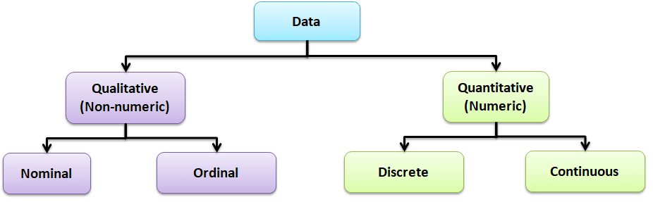
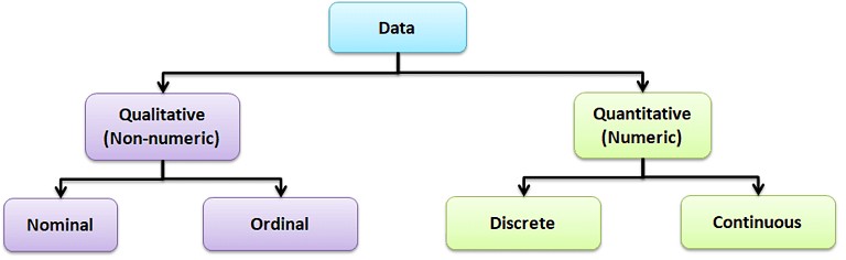
Data is a set of values that can be either qualitative or quantitative. It may be a number, a measurement, an observation, or even a description.

Qualitative data: Qualitative data, also known as non-numeric data, essentially describes the traits of a value or data point. It consists of a finite number of possible categories into which each data point may fall.

Types of Qualitative Data

  • Nominal data: A type of descriptive data with more than two categories; it can refer to the names or labels of the data points. For example, Hair color: black, brown; Gender: male or female.
  • Ordinal data: Ordinal data provides good information about the order of choices. In other words, it arranges information in a particular order without indicating a specific relationship between items. Example: pass or fail, customer service, good or bad, etc.

Quantitative data: It is also known as numerical data. The data points are counts or measurements. Unlike Qualitative data, it consists of an infinite number of possible categories into which each data point may fall. The Quantitative data is further divided into two data types:

  • Discrete data: The data is discrete if the measurements are whole numbers or counts. For example, the number of customer complaints, weekly defects data, etc.
  • Continuous data: The data is continuous if the measurement takes on any value, usually within some range. For example, Stack height, distance, cycle time, etc.

Discrete Data

Discrete data comprises distinct, separate values with clear boundaries between each possible value. It assumes specific, individual values and cannot be infinitely subdivided. Typically, discrete data is counted and often represented by whole numbers. Examples: Number of defects in a product, or number of red balls in a bowl.

Discrete Data analysis tools

Discrete data analysis involves techniques specifically tailored for data that consists of distinct, countable values. Here are some common tools used for analyzing discrete data:

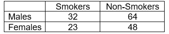
Contingency Table

A contingency table, also known as cross-tabulation or a two-way frequency table, typically summarizes and analyzes the relationship between two categorical variables. Contingency tables are a type of table in a matrix format that displays the frequency distribution of the variables. In other words, contingency tables represent a 2-way classification table containing frequencies of how often things appear, and they can determine if two variables are independent or significantly associated.

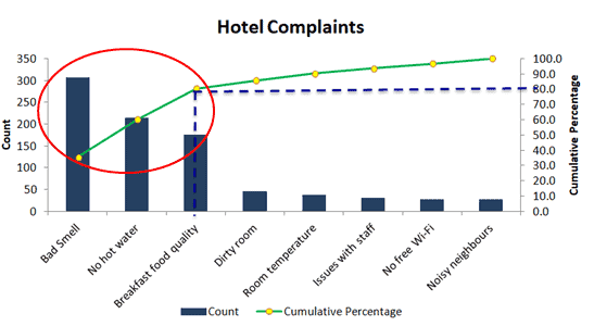
Pareto Chart

The Pareto Chart (Pareto Diagram) is a graphical tool that maps and grades business process problems from the most recurrent to the least frequent. In other words, it helps identify the most frequently occurring problems or separates the vital few from the trivial many. The Pareto Chart combines both a bar chart and a line chart. The bar chart shows the frequency of occurrence or defects, while the line graph displays the cumulative data percentage in descending order.

Attribute charts are a kind of control chart to display information about defects and defectives. They help you visualize the enemy: variation!

Defect:

A defect is a non-conformity that does not meet the customer’s requirements. A product or service may have one or more defects but is defective only if defects prevent the product from functioning.

Defect analysis is carried out based on the Poisson distribution (evaluates the rate of defects in the process) using the following methods.

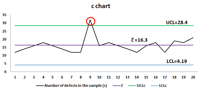
c chart: c chart also known as the control chart for defects (counting the number of defects), is generally used to monitor the number of defects in constant-sized units. There may be a single type of defect or several different types, but the c-chart tracks the total number of defects in each unit, assuming that the underlying data approximate the Poisson distribution. 

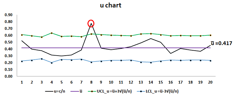
u chart: u chart is also known as the control chart for defects per unit chart. It is generally used to monitor the count type of data where the sample size is greater than one. There may be a single type of defect or several different types, but the u chart tracks the average number of defects per unit, and it assumes the underlying data approximate the Poisson distribution.

Defective:

A product or service that has one or more defects and it is not suitable for use. In other words, a product or service is defective if the defect(s) existing in it affects its functionality.

Using the following methods, a defective analysis is carried out based on Binomial distribution (evaluates the proportion of defectives in the process).

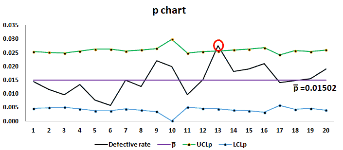
p chart: p chart is also known as the control chart for proportions. It is used to analyze the proportions of non-conforming or defective items in a process.  It uses a Binomial Distribution to measure the proportion of defective or non-conforming units in a sample.

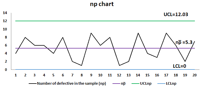
np chart: np chart is also known as the control chart for defectives (d-chart). It generally monitors the number of non-conforming or defective items in the measurement process.  It uses binomial distribution to measure the number of defective or non-conforming units in a sample. An np chart is very similar to a p chart. np chart plots the number of items, while the p chart plots the proportion of defective items.

Continuous Data

Continuous data encompasses values that can take on any value within a given range and allows measurement to any level of precision. It is characterized by its infinite divisibility, lacking clear boundaries between adjacent values. Measurements or observations represented in fractional or decimal form fall under continuous data.

Examples: Height, weight, temperature, time, etc.

Continuous Data Analysis tools

Statistical techniques and tools often specifically address data capable of assuming any value within a given range in continuous data analysis. Following are the Continuous data analysis tools.

Data Analysis

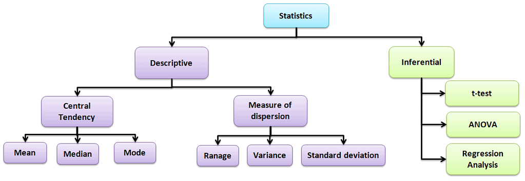
Descriptive statistics

Values that describe the traits of the sample or population. In other words, it provides a simple summary of the sample and the measures.

Central Tendency

Refers to the statistical measure used to determine the center of a distribution of a data set. Based on the situation, the measure of central tendency could be either Mean, Median, or Mode.

  • Mean: The mean is the total of all data values divided by the number of data points.
  • Median: The median is the middle value when the data is arranged in order from least to greatest or vice versa. If the data set has even values, the median is the average of the middle two values.
  • Mode: The mode is the value that often occurs in the data set.

Measure of dispersion

Dispersion is the degree of variation in the data. Dispersion measures the extent to which different items tend to disperse from the central tendency.

Different types of measures of dispersion

Range: Range is the difference between the maximum and the minimum value.

Variance: Variance measures the dispersion of a set of data points around their mean value.

Standard Deviation: Standard deviation is the most popular measure of dispersion. The main purpose is to measure the amount of variation in a process. One of the most common measures of variability in a dataset or population is the Standard Deviation.

 Box-and-Whisker Plot

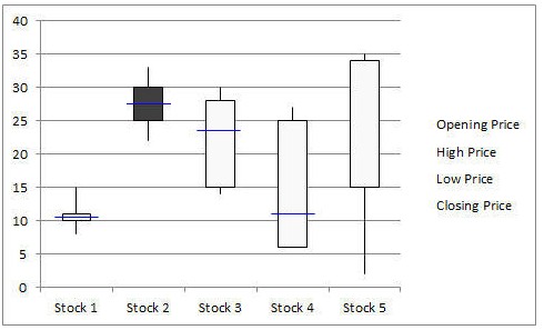
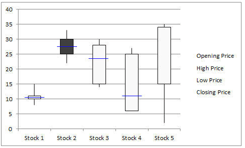
Box-and-Whisker plot, also known as a Box and Whisker plot, is a pictorial representation of continuous data. Box plots show the Max, Min, median, interquartile range Q1, Q3, and outlier data.

Data Analysis

Run Chart

Run charts, also known as Time Series Plots, plot data over time using line graphs. They help to identify the pattern of the data in the time series. Because they don’t use control limits, we cannot judge whether the process is stable or not. However, run chat shows how the process is behaving. The advantage of the run chart is that it identifies the special cause(s) in a process.

Data Analysis

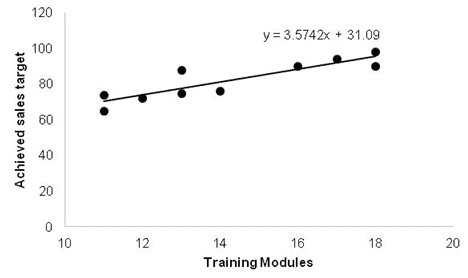
Scatter Diagram

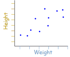
Scatter diagrams, also known as Correlation Charts or XY Graphs, plot the relationship between two continuous variables. These can include the independent variable on the x-axis and the dependent variable on the y-axis.

Data Analysis

Histogram

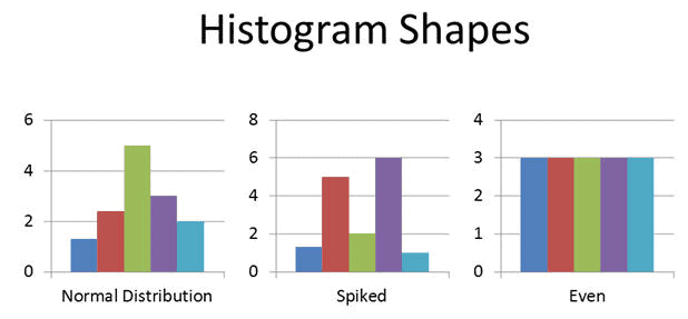
A Histogram is the graphical representation of a frequency distribution. It is in the form of a rectangle with class intervals as the base and the corresponding frequencies as the height. Particularly, there are no gaps between any two successive rectangles.

Normal Probability Plot

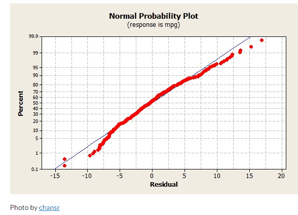
The Normal Probability Plot is a graphical method to assess whether the data set follows a normal distribution or not. This includes identifying outliers, skewness, etc. Furthermore, the Normal Probability Plot is one example of a Quantile-Quantile (Q-Q) plot.

Data Analysis

Regression Analysis

A Regression Analysis is a method for assessing relationships between variables by examining system behavior. Researchers employ various analysis techniques to determine the relationship between dependent and independent variables, with Regression Analysis standing out as one of the most effective. For example, they can utilize transformations to mitigate higher-order terms within the model.

ANOVA

Analysis of Variance (ANOVA) is a parametric statistical technique used to compare data sets. This technique was invented by R.A. Fisher; hence, it is also referred to as Fisher’s ANOVA. It is similar to techniques such as t-test and z-test to compare means and also the relative variance between them.

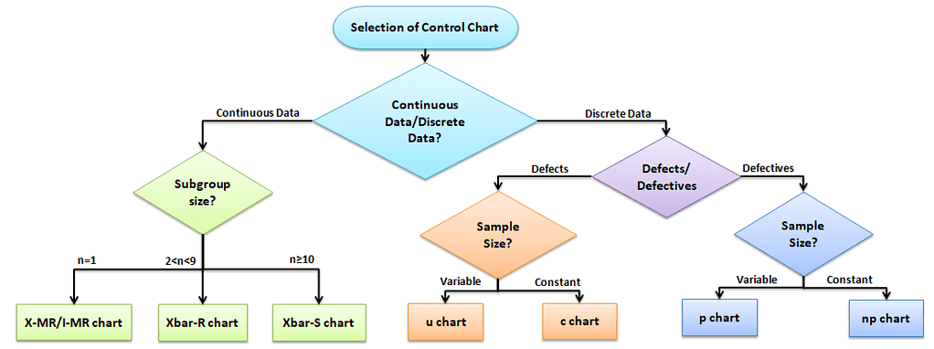
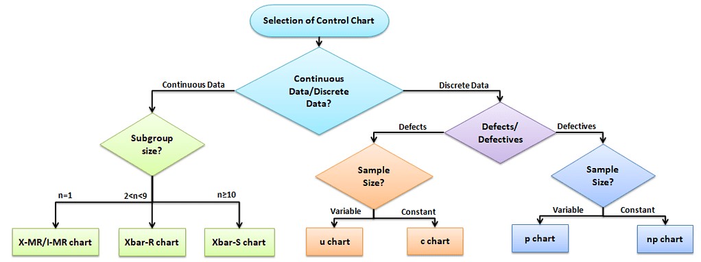
Data Analysis: Selection of Control chart for Discrete Data and Continuous Data

The control chart is a graph used to study how a process changes over time. A control chart always has a central line for the average, an upper line for the upper control limit, and a lower line for the lower control limit. The control limits are ±3σ from the centerline.

Selection of an appropriate control chart is very important in control chart mapping, otherwise ended up with inaccurate control limits for the data.

X̅ and R charts charts use measurable quantities such as length, weight, and height. Attribute control charts use attribute data. In other words, the data that counts the number of defective items or the number of defects per unit.

Advantages of Data Analysis

  • Data analysis identifies inefficiencies and areas for improvement, enabling targeted problem-solving.
  • Insights from data drive efficiency improvements, cost reductions, and resource optimization efforts.
  • Data analysis supports evidence-based decision-making
  • Analysis helps to get insights from data, trends, correlations, and predictive patterns.
  • Data Analysis identifies and mitigates risks by examining historical data and helps to predict potential issues.
  • Understanding customer data informs tailored strategies to meet customer needs and preferences effectively.
  • Data Analysis tracks progress, evaluates performance against metrics, and assesses intervention effectiveness.

Using Data to Make Better Decisions

Great TED presentation on using data to make better decisions.


Basic Six Sigma Statistics

Basic Six Sigma statistics is the foundation for Six Sigma projects. It allows us to describe the data that makeup processes X and Y in terms of numbers. Today, statistics is an important part of the day-to-day activities of any organization. Numbers and data play a vital role in Six Sigma projects; hence Six Sigma professionals and other stakeholders must have basic Six Sigma statistics knowledge.

Data Types

Data is a set of values that can be either qualitative or quantitative. It may be a number, a measurement, an observation, or even a description.

Basic Six Sigma Statistics

Qualitative data: Qualitative data, also known as non-numeric data, is basically data that describes the traits of a value or data point. It is made of a finite number of possible categories into which each data point may fall.

Types of Qualitative data

  • Nominal data: A type of descriptive data with more than two categories; it can refer to the names or labels of the data points. For example, Hair color – black, brown; Gender – male or female.
  • Ordinal data: Ordinal data provides good information about the order of choices. In other words, it arranges information in a particular order without indicating a specific relationship between items. Example: pass or fail, customer service, good or bad, etc.

Quantitative data: It is also known as numerical data. The data points are counts or measurements. Unlike Qualitative data, it consists of an infinite number of possible categories into which each data point may fall. The Quantitative data is further divided into two data types:

  • Discrete data: The data is discrete if the measurements are whole numbers or counts. For example, the number of customer complaints, weekly defects data, etc.
  • Continuous data: The data is continuous if the measurement takes on any value, usually within some range. For example, Stack height, distance, cycle time, etc.

Population Parameters

Population parameters refer to the characteristics of a population. In other words, it describes some aspect of the population. These are used to make inferences about a larger group based on a smaller sample.

Sample Statistics

Sample statistics are measures calculated from a sample of individuals that are used to estimate or make inferences about the population parameters.

Furthermore, sample statistics is to estimate the population parameters, as it is often impossible or impractical to measure the characteristics of an entire population. The accuracy of the estimates obtained from sample statistics depends on the sample size and how the sample was selected from the population. Larger sample sizes generally lead to more accurate estimates of the population parameters.

A few common population parameters and sample statics are:

Mean: The mean is the average value of a variable in a population or sample. It is calculated by adding all data values divided by the number of data points.

Standard Deviation: Standard deviation is the most popular measure of dispersion. It is used to measure the amount of variation in a process. It indicates how much the individual values in a population or sample deviate from the population mean.

Proportion: The proportion is the number of individuals in a population or sample who holds a certain characteristic divided by the total number of individuals in the population or sample. For example, the proportion of male in a population or sample would be the number of males divided by the total population or sample.

Variance: Variance measures the dispersion of a set of data points around their mean value. It is calculated by taking the average of the squared differences of each value from the population or sample mean.

Distinguish between population parameters and sample statistics
  • Population parameters are descriptive measures that summarize a characteristic of a whole population. Whereas, Sample statistics, are descriptive measures that summarize a characteristic of a sample from a population.
  • Population parameters are fixed and constant, while sample statistics can vary depending on the sample selected from the population.
  • Population parameters are typically of greater interest to researchers than sample statistics, as they provide a more accurate description of the population.
  • Since it is often impractical to measure characteristics of an entire population, sample statistics are important in helping to make inferences about the population.

Basic Types of Statistics used in Six Sigma

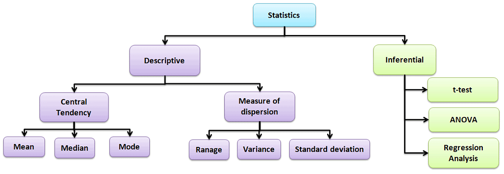
Statistics are made of principles and methodologies for collecting, analyzing, interpreting, and presenting data in a meaningful way. Statistics helps to understand the data behavior, identify improvement opportunities, and predict future process performance.

Types of statistical analysis:

Basic Six Sigma Statistics

Descriptive statistics

Values that describe the traits of the sample or population. In other words, it provides a simple summary of the sample and the measures.

Central Tendency

Refers to the statistical measure used to determine the center of a distribution of a data set. Based on the situation, the measure of central tendency could be either Mean, Median, or Mode.

  • Mean: The mean is the total of all data values divided by the number of data points.
  • Median: The median is the middle value when the data is arranged in order from least to greatest or vice versa. If the data set has even values, the median is the average of the middle two values.
  • Mode: The mode is the value that often occurs in the data set.

Measure of dispersion

Dispersion is the degree of variation in the data. Dispersion measures the extent to which different items tend to disperse from the central tendency.

Different types of measures of dispersion

Range: Range is the difference between the maximum and the minimum value.

Variance: Variance measures the dispersion of a set of data points around their mean value.

Standard Deviation: Standard deviation is the most popular measure of dispersion. Main purpose is to measure the amount of variation in a process. Standard Deviation is one of the most common measures of variability in a data set or population.

Kurtosis: Kurtosis is a statistical measure to determine whether the data is heavy-tailed or light-tailed relative to a normal distribution.  In other words, it is a measure of the thickness of the tails of a distribution.

Inferential statistics:

The purpose of Inferential statistics is to draw conclusions or inferences about the traits of a population based on data from a sample. In other words, using probability to learn about a population parameter from information given in a sample. T-tests, regression analysis, and Analysis of variance (ANOVA) are a few examples of Inferential statistics.

Shape of the distribution

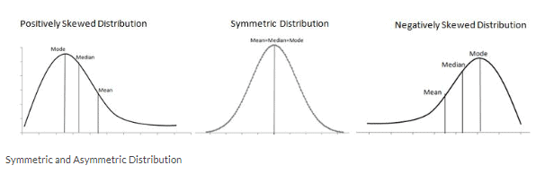
The shape of data distribution is shown by its number of peaks and by the symmetry possession, skewness, or uniformity. Skewness is a measure of the lack of symmetry. In other words, skewness is the measure of how much the probability distribution of a random variable deviates from the Normal Distribution.

Symmetrical Distribution: Generally, symmetrical distribution appears as a bell curve. The perfect normal distribution is the probability distribution that has zero skewness. Symmetrical distribution occurs when mean, median, and mode occur at the same point, and the values of data points occur at regular frequencies. 

Positively Skewed Distribution: A distribution is said to be skewed to the right if it has a long tail that trails toward the right side. The skewness value of a positively skewed distribution is greater than zero.

Negatively Skewed Distribution: A distribution is said to be skewed to the left if it has a long tail that trails toward the left side. The skewness value of a negatively skewed distribution is less than zero.

Summarizing the data

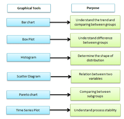
Graphical analysis is one of the best ways to summarize the data in Six Sigma projects. It creates pictures of the data, which will help understand the patterns and the correlation between process parameters. Often, graphical analysis is the starting point for any problem solving method.

Different graphical analysis methods:

Box-and-Whisker plot, also known as Box and Whisker plot, is a pictorial representation of continuous data. The box plot shows the Max, Min, median, interquartile range Q1, Q3, and outlier.

A run chart is also known as a time series plot. It is a line graph of data plotted over time. It helps to identify the pattern of the data in the time series. Because they don’t use control limits, we cannot judge whether the process is stable or not.

Pareto Chart, also known as 80-20 rule. It is a combination of a bar chart and a line chart. The actual data is in descending order using a bar chart, and the cumulative data is in ascending order using a line graph.

Helpful Basic Six Sigma Statistics Videos

Six Sigma Symbols

s (or sd): The sample standard deviation is a point estimate for the population standard deviation / the dispersion statistic for samples

µ: the central tendency statistic for populations

XBar: a point estimate for the population mean

σ: the actual population standard deviation for the measurement of dispersion in a population

N is for populations

n: The statistic for number of data in a sample

x:  the individual value

Basic Six Sigma Statistics References

Statistics Guides:

When you’re ready, there are a few ways I can help:

First, join 12,000+ other Six Sigma professionals by subscribing to my email newsletter. A short read every Monday to start your work week off correctly. Always free.

* * *

If you’re looking to pass your Six Sigma Green Belt or Black Belt exams, I’d recommend starting with my affordable study guide:

1)→ 🟢Pass Your Six Sigma Green Belt: a study guide organized by the exam Body of Knowledge, 1,000+ practice questions with detailed answer explanations, and 8 full-length mock exams

2)→ ⚫Pass Your Six Sigma Black Belt: the full Black Belt Body of Knowledge, 2,000+ practice questions with detailed answer explanations, and 8 full-length mock exams

You’ve spent so much effort learning Lean Six Sigma. Why leave passing your certification exam up to chance? This comprehensive study guide offers 1,000+ exam-like questions for Green Belts (2,000+ for Black Belts) with full answer walkthroughs, access to instructors, detailed study material, and more.

​ Thousands have used this system to prepare. Join them here. 
Process Performance Pp and Ppk

Process Capability

How do you know if your process is capable? Process Capability Pp measures the process spread vs. the specification spread. In other words, how distributed the outcome of your process is vs. what the requirements are.

If you’d like more depth, including calculations, etc., see these articles:

Note: Use Pp & Ppk when you are initially setting up your process. After a process has reached statistical control, use Cp & Cpk.

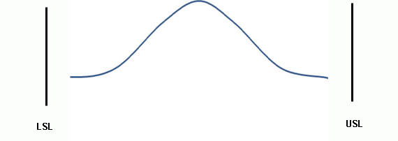
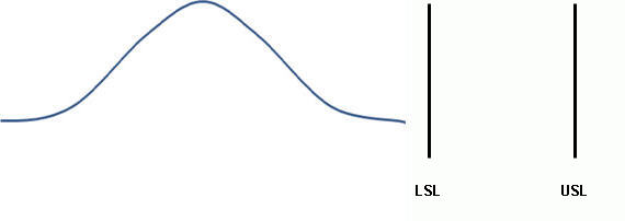
Let’s imagine that your process has 2 specifications; a Lower Specification Limit (LSL) which is the lowest value allowed, and an Upper Specification Limit (USL), the highest value allowed.  We call the difference between the two the specification spread, sometimes referred to as the Voice of the Client.

The process spread is the distance between the highest value generated and the lowest. We sometimes refer to this as the Voice of the Process.

Process Spread vs. Specification Spread

Think of the Specification Spread as the sides of your garage – those are static, they are not moving, and it is important that your process puts values inside those bounds. The Process Spread is the size of the car you are trying to fit in.

Specification Spread vs Process Spread: Process Performance (Pp, Ppk)
Specification Spread vs Process Spread

Can A Process Meet Specifications?

The answer is in the amount of variation in your process. If your process spread exceeds the specification spread, then the answer is no.  However, if the process spread is less than the specification spread, then process variation is low enough for it to fit.

Process Meets Specifications: Good Potential Performance

good potential performance

Process Does NOT Meet Specifications: Bad Potential Performance

Bad Potential Performance: Process Performance (Pp, Ppk)
Bad Potential Performance
This is what happens when your specification spread does not match your specification spread!
This is what happens when your process spread does not match your specification spread!

Calculating Process Capability (Pp)

Pp = (USL – LSL) / 6 * s : where “s: the standard deviation, or the ‘fatness’ or dispersion of the bell curve.

What is a ‘Good’ Process Capability (Pp) Number?

According to Six Sigma, we want a Pp of above 1.5 because that would reflect a process with less than 3.4 DPMO – the definition of 6 Sigma quality.

How do we come to that?

Well, we want to have 6 sigmas (standard deviations) between the mean of the process and the LSL. Since a normal distribution is symmetric, that means we also want 6 sigmas between the mean and the USL. That’s a total of 12 sigmas between the USL and LSL.

In other words, USL – LSL should = 12 for us to reach 6 σ quality standards of 3.4 DPMO.

See how that is reflected in the equation Pp = (USL – LSL) / 6* s?

Let’s replace (USL – LSL) with 12:      Pp = (USL – LSL) / 6* s   = 12 σ / 6 * s = 2 σ / s

Process Capability Index

Is the Process Acceptable? Ppk (Capability)

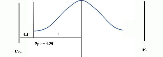
Ppk is another performance index that measures how close the current process means proximity is to the specification limits. In other words, does this process deliver acceptable results?

We tell this by trying to see how centered the process is. If the process is not centered well, it is deemed not acceptable.

That Process was poorly centerned! Unacceptable! An unsuccessful Process Performance (Pp, Ppk).
That process was poorly centered! Unacceptable!

Calculating Ppk

There are two ways to calculate Ppk, depending on how your process aligns.

Actual performance Ppk: Process Performance (Pp, Ppk)
Actual performance Ppk

Process Mean close to USL

If your Process Mean (central tendency) is closer to the USL, use Ppk =  [ USL – x(bar) ] / 3 s, where x(bar) is the Process Mean.

Process Mean close to LSL

If your Process Mean (central tendency) is closer to the LSL, use Ppk =  [x(bar) – LSL ] / 3 s, where x(bar) is the Process Mean.

Interpreting Ppk Scores

A Ppk of 1 means that there is “half of a bell curve” between the center of the process and the nearest specification limit. That means your process is completely centered.

Pp, Ppk In Relation to Z Scores

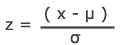
Ppk can be determined by dividing the Z score by three. A z score is the same as a standard score; the number of standard deviations above the mean.

z_pop

Z = x – mean of the population / standard deviation.

Ppk = ( USL – µ) / 3σ = z / 3

ASQ Six Sigma Green Belt Process Performance Questions

Question: Which of the following measures is increased when process performance is improved?

(A) Variability range
(B) Capability index
(C) Repeatability index
(D) Specification limits

Answer:

Unlock Additional Members-only Content!

To unlock additional content, please upgrade now to a full membership.
Upgrade to a Full Membership
If you are a member, you can log in here.

Process Capability (Cp & Cpk)

Cp and Cpk are considered short-term potential capability measures for a process. In Six Sigma, we want to describe the process quality in terms of sigma because this gives us an easy way to talk about how capable different processes are using a common mathematical framework. In other words, it allows us to compare an apple process to an orange process!

Process Capability

This is a long article, but I thought it was important to keep Cp and Cpk together. First, I’ll address Cpk, then Cp. There are also crib notes on what the equations mean in a real performance sense, what you should be able to tell about a process depending on Cp and Cpk values, and more. Please let me know in the notes below if you do not find what you are looking for.

Before We Begin!

I wrote this article to help Six Sigma Green Belt and Black Belt candidates prepare for and pass their exams.

If that’s you, leave me a comment below or contact me and let me know which organization and belt you’re studying for. This will help me make the article even better for you.

If you’re studying for something else, please leave a comment or contact me and let me know what you are studying for. Again, this will help me improve the article for you and everyone else. Thanks, Ted.

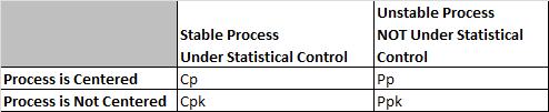
What is the Difference between Cp, Cpk and Pp, PPk?

Cp Cpk vs Pp Ppk
Cp Cpk vs Pp Ppk

Cp and Cpk are called Process Capability. Pp and Ppk are called Process Performance. In both cases, we want to try to verify if the process can meet Customer CTQs (requirements).

Cp and Cpk are used for Process Capability. Generally, you use this when a process is under statistical control. This often happens with a mature process that has been around for a while. Process capability uses the process sigma value determined from either the Moving Range, Range, or Sigma control charts.

Pp and PPk are used for Process Performance. Generally, you use this when a process is too new to determine if it is under statistical control. Ex. you are piloting a new process or testing a short pre-production run. Because there is not a lot of historical data, we take large samples from the process to account for variation. Process Performance generally uses sample sigma in its calculation.

In theory, Cpk will always be greater than or equal to Ppk. There are anomalies seen when the sample size is small, and the data represents a short amount of time where estimating using R will overstate standard deviation and make Cpk smaller than Ppk. It is not real; there can never be less variation in the long term since the long term is using all of the data, not just two pieces of data from every subgroup.

Evaluating process capability with Cp & Cpk mirrors what is done (and why it is done) when following the Pp & Ppk approach. The main difference is that you use Cp & Cpk after a process has reached stability or statistical control.

Cpk vs. Ppk

Ppk tells us how a process has performed in the past, and you cannot use it to predict the future because the process is not in a state of control.

If a process is under statistical control;

The values for Cpk and Ppk will converge to almost the same value because the sigma and the sample standard deviation will be identical (use an F test to determine).

In other words, if Cpk == Ppk, the process is likely in statistical control.

If a process is NOT in statistical control;

Cpk and Ppk values will differ distinctly, perhaps by a very wide margin.

What is the Difference Between Cp and Cpk?

Cp vs. Cpk

Cp and Cpk measure your consistency compared to your average performance.

The ‘k’ stands for ‘centralizing factor.’ The index considers the fact that your data may not be centered.

Cpk tells us what a process can do in the future, assuming it remains in a state of statistical control.

The Shooting at a Target Analogy

In a perfectly centered data set, there will be no difference between Cp and Cpk. Think of throwing darts at a dart board and having the center of the bull’s eye be the 0,0 on a cartesian plane and the edges being out three units from that center point (we will use the edge of the dartboard or 3 and -3 as our USL and LSL). In a perfectly centered sample of darts, your average distance from the center, or Mu, will be 0. A little algebra will show us that your Cpk and Cp numbers are the same. Min((0- -3)/3s , (3-0)/3s) = (3- -3)/6s = 1s .

Things get a little harrier when the darts move up, say to be centered at an average of 2 units above center. Now you end up with a Cpk of (3-2)/3s = 1/3s, but your Cp is still the same 1s as before. It is important to note that because Cpk uses the minimum function, it will always be equal to or smaller than the Cp for the same set of data.

What is Cpk?

The Parking a Car in the Garage Analogy

Think of the walls of your garage – where you have to fit your car – they become the customer specification limits. If you go past those limits, you will crash, and the customer will not be happy!

When your process has a lot of variation, the process average is all over the place. Not good for parking a car or any other process. To give your parking process the best chance of success, you should reduce variation and centering.

If the car is too wide for the garage, nothing you do to center the process will help. You have to change the dispersion of the process (make the car smaller.)

If the car is a lot smaller than the garage, it doesn’t matter if you park it exactly in the middle; it will fit, and you have plenty of room on either side. That’s one of the reasons the Six Sigma philosophy focuses on removing variation in a process.

If you have a process that is in control and with little variation, you should be able to park the car easily within the garage and thus meet customer requirements. Cpk tells you the relationship between the car’s size, the garage’s size, and how far away from the middle of the garage you parked the car.”

Preparing for a Six Sigma exam? Get the one-page Cp, Cpk, Pp, Ppk cheat sheet.

Formulas, how to judge the number, the exam rules, and a worked example on one printable page. Enter your email and I'll send it now.

You'll also get my weekly Six Sigma newsletter. Unsubscribe anytime.

How to Calculate Cpk

Cpk is a measure to show how many standard deviations the specification limits are from the center of the process. On some processes, you can do this visually. Others require an equation.

To find Cpk you need to calculate a Z score for the upper specification limit (called Z USL) and a Z score for the lower specification limit (called Z LSL).

Since we are trying to measure how many standard deviations fit between the center line and the specification limit, you should not be surprised that the value of those limits, the process mean, and the standard deviation are all components of the Z calculation.

Cp is an abbreviation. There are two parts, the upper and the lower denoted Cpu and Cpl, respectively. Their equations are:

Cpl = (Process Mean – LSL)/(3*Standard Deviation)
Cpu = (USL – Process Mean)/(3*Standard Deviation)

Cpk is merely the smallest value of the Cpl or Cpu denoted:  Cpk= Min (Cpl, Cpu)

Why are we dividing by 3 to find Cpk?

We know that any specification limit has an upper and lower bound. Because you know that 6 sigmas (or six standard deviations) account for nearly all eventualities in a process (assuming normal distribution), you shouldn’t be surprised to see the “/ 3” because we are looking at only one side of the distribution.

Calculating Cpk using a Z Value

If you have a Z value, the equation is very easy;

Cpk can be determined by dividing the Z score by three.

A z score is the same as a standard score; the number of standard deviations above the mean.

z_pop

Z = x – mean of the population / standard deviation.

Notes and Characteristics of Cpk

Cpk and Centered Processes

If a process is perfectly centered, it has a Cp of 1. That would indicate that the mean was 3 standard deviations away from the upper limit and the lower limit.

A perfectly centered process is a process that has a mean exactly in between the 2 specification limits (meaning halfway between the two will have a Cpk of 1. How is this possible? Let’s check the math.

If a process is perfectly centered, then we know that the (USL – Process mean) equals the same thing as the (Process Mean – LSL). Let’s call that A.

Z USL = USL – Process Mean / Standard Deviation. then becomes Z USL = A/ Standard Deviation

Z LSL = Process Mean – LSL / Standard Deviation then becomes Z LSL = A / Standard Deviation.

The exact same thing.

Notes on Cpk

  • Cpk measures how close a process is performing compared to its specification limits and accounting for the natural variability of the process.
  • Larger is better. The larger Cpk is, the less likely it is that any item will be outside the specification limits.
  • When Cpk is negative, it means that a process will produce output that is outside the customer specification limits.
  • When the process’s mean is outside the customer specification limits, the value of Cpk will be negative.
  • To satisfy most customers, we generally want a Cpk of at least 1.33 [4 sigmas] or higher.
  • Cpk can have an upper and lower value reported.
    • If the upper value is 2 and the lower is 1, we say it has been shifted to the left.
    • This tells us nothing about whether the process is stable or not.
    • We must report the lower of the 2 values.
Process Capability Cp Cpk example
That was poorly centered!

What are Good Values for Cpk?

Remember the Car parking in the garage analogy?

  • Cpk = Negative number: Your process will regularly crash the car into the wall.
  • Cpk =0.5: You have a good chance of hitting the wall on entry.
  • Cpk =1:  Your car may be just touching the nearest edge of the entry.
  • Cpk =2: Great! You have great clearance. You could double the width of your car before you hit the side of the garage.
  • Cpk =3: Excellent!  You have excellent clearance. You could triple the width of your car before you hit the side of the garage.

How to Calculate Cp

Just as you use Cp & Cpk when a process is stable and Pp & Ppk when a process is new, the way you calculate each is a bit different, too.

Let’s revisit Pp

Pp = (USL – LSL) / 6* s

In Pp, s is the standard deviation or the ‘fatness’ or dispersion of the bell curve.

In Cp, we replace s with an estimate of σ we call σr. To do that, we use the Moving Range concept from a Moving R Bar chart or an XMR Chart. So, σr = [ R Bar  / d2]

R Bar comes from the Moving range.

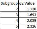
D2 reflects values derived from integrating the area under the normal curve. We often use a table that gives a d2 value based on the subgroup size (n, the number of measurements in each subgroup), not on how many subgroups were collected.

d2 subgroup values
d2 subgroup values

Cp does not account for centering.

First, Cp = (USL – LSL) / ( 6*  σr  )

Second, Cp = (USL – LSL) / ( 6*  R Bar  / d2 )

Cp for Process Mean close to USL

If your Process Mean (central tendency) is closer to the USL, use:    [ USL – x(bar) ] / [3 *  R Bar  / d2], where x(bar) is the Process Mean.

Cp for Process Mean close to LSL

If your Process Mean (central tendency) is closer to the LSL, use:    [x(bar) – LSL ] / [3 *  R Bar  / d2], where x(bar) is the Process Mean.

Capability Index

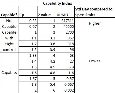
How do Cp, Z values, DPMO, Specification Limits, Standard Deviation, and Capability all relate?

Also, see Z values and process capability.

Capability Index
Capability Index

Notes on Cp Values

  • If the ratio is greater than one, then the Engineering Tolerance is greater than the Process Spread, so the process has the “potential” to be capable (depending on process centering).
  • If the Process Spread is greater than the Engineering Tolerance, then the process variation will not “fit” within the tolerance, and the process will not be capable (even if the process is centered appropriately).

Capability Ratio Cr

The capability ratio is the inverse of Cp

Cr = 1/ Cp =  ( 6*  σr  ) /  (USL – LSL)

If Cr < 0.75, the process is capable.

If Cr = 0.75 – 1.00, the process is capable of tight control.

When the Cr >1, the process is not capable.

Notes on Relating Cp And Cpk

  • If Cp == Cpk, then the process is perfectly centered. If perfectly centered, Cp == Cpk.
  • Because Cpk accounts for centering (where Cp does not), Cpk can never be larger than Cp.
  • Both assume a stable process.

Process Capability Videos

Cpk Videos

Great, clear, concise video on this subject.

“If you were producing a Cpk equal to 1, then you could expect to produce at least 99.73% good parts.”

Lecture on Process Capability and SPC

ASQ Six Sigma Black Belt Certification Process Capability Questions:

Question: Data being used in the initial set-up of a process is assumed to have a normal distribution. If the nominal (target) is set at the center of the distribution, and the specification limits are set at ±3s from the center, then the Cpk is equal to:

(A) -0.25
(B) 1.00
(C) 1.33
(D) 1.67

Answer:

Unlock Additional Members-only Content!

To unlock additional content, please upgrade now to a full membership.
Upgrade to a Full Membership
If you are a member, you can log in here.

ASQ Six Sigma Green Belt Certification Process Capability Questions:

Question: When calculating the Cp index, what does the standard deviation represent in the formula Cp = (USL – LSL) / 6σ?

(A) The tolerance interval
(B) The confidence interval for the result
(C) The range of the process
(D) The variance of the index

Answer:

Unlock Additional Members-only Content!

To unlock additional content, please upgrade now to a full membership.
Upgrade to a Full Membership
If you are a member, you can log in here.

When you’re ready, there are a few ways I can help:

First, join 12,000+ other Six Sigma professionals by subscribing to my email newsletter. A short read every Monday to start your work week off correctly. Always free.

* * *

If you’re looking to pass your Six Sigma Green Belt or Black Belt exams, I’d recommend starting with my affordable study guide:

1)→ 🟢Pass Your Six Sigma Green Belt: a study guide organized by the exam Body of Knowledge, 1,000+ practice questions with detailed answer explanations, and 8 full-length mock exams

2)→ ⚫Pass Your Six Sigma Black Belt: the full Black Belt Body of Knowledge, 2,000+ practice questions with detailed answer explanations, and 8 full-length mock exams

You’ve spent so much effort learning Lean Six Sigma. Why leave passing your certification exam up to chance? This comprehensive study guide offers 1,000+ exam-like questions for Green Belts (2,000+ for Black Belts) with full answer walkthroughs, access to instructors, detailed study material, and more.

​ Thousands have used this system to prepare. Join them here.