Data distribution is a function that specifies all possible values for a variable and also quantifies the relative frequency (probability of how often they occur). Distributions are considered to be any population that has a scattering of data. It’s important to determine the population’s distribution so we can apply the correct statistical methods when analyzing it.
Data distributions are widely used in statistics. Suppose an engineer collects 500 data points on a shop floor. It does not give any value to the management unless they categorize or organize the data in a useful way. Data distribution methods organize the raw data into graphical methods (like histograms, box plots, run charts, etc.) and provide helpful information.
The basic advantage of data distribution is to estimate the probability of any specific observation in a sample space. A probability distribution is a mathematical model that calculates the probability of occurrence of different possible outcomes in a test or experiment. We use them to define different types of random variables (typically discreet or continuous) to make decisions, depending on the models. One can use mean, mode, range, probability, or other statistical methods based on the random variable category.
Types of Distribution
Distributions are basically classified based on the type of data (Typically discreet or continuous)
Discrete Distributions
A discrete distribution results from countable data with a finite number of possible values. Furthermore, we can report discrete distributions in tables, and the respective values of the random variable are countable. Ex: rolling dice, choosing several heads, etc.
Probability mass function (pmf): A probability mass function is a frequency function that gives the probability for discrete random variables, also known as the discrete density function.
Simply Discrete= counted
Different types of discreet distributions are
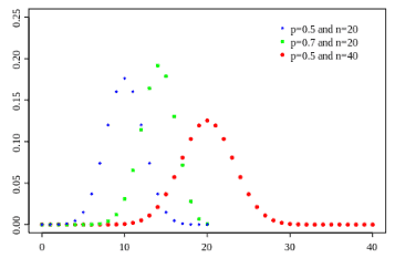
Binomial distribution
- The binomial distribution measures the probability of the number of successes or failure outcomes in an experiment on each try.
- Characteristics are classified into two mutually exclusive and exhaustive classes, such as the number of successes/failures and the number accepted/rejected that follow a binomial distribution.
- Ex: Tossing a coin: The probability of the coin landing Head is ½, and the probability of the coin landing tail is ½
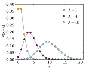
Poisson distribution
- The Poisson distribution is the discrete probability distribution that measures the likelihood of a number of events occurring in a given period when the events occur one after another in a well-defined manner.
- Characteristics that can theoretically take large values but actually take small values have Poisson distribution.
- Ex: Number of defects, errors, accidents, absentees, etc.
Hypergeometric distribution
- The hypergeometric distribution is a discrete distribution that measures the probability of a specified number of successes in (n) trials without replacement from a relatively large population (N). In other words, sampling without replacement.
- The hypergeometric distribution is similar to the binomial distribution;
- The basic difference of binomial distribution is that probability of success is the same for all trials, while it is not the same case for hypergeometric distribution.
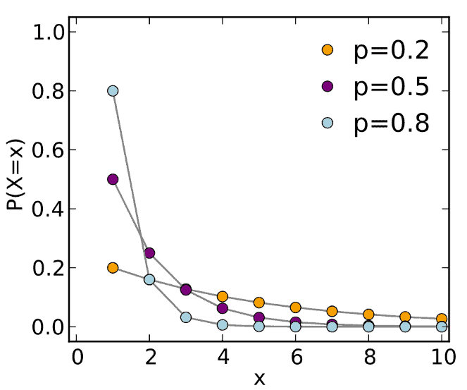
Geometric distribution
- The geometric distribution is a discrete distribution that measures the likelihood of when the first success will occur.
- An extension of it may be considered a negative binomial distribution.
- Ex: Marketing representative from an advertising agency randomly selects hockey players from various universities until he finds a hockey player who attended the Olympics.
Continuous Distributions
A continuous distribution contains infinite (variable) data points, which it displays on a continuous measurement scale. A continuous random variable is a random variable with a set of possible values that is infinite and uncountable. It measures something rather than just counting; we typically describe it using probability density functions (pdf).
Probability density function (pdf): The probability density function describing the behavior of a random variable. It is normally grouped frequency distribution. Hence probability density function sees it as the ‘shape’ of the distribution.
Simply Continuous = can take many different values
Different types of continuous distributions are
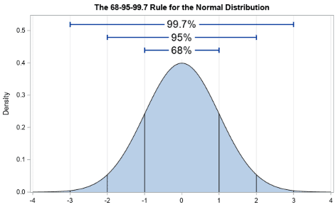
Normal Distribution
- Some people also refer to normal distributions as Gaussian distributions. It is a symmetrical bell shape curve with higher frequency (probability density) around the central value. The frequency sharply decreases as values are away from the central value on either side.
- In other words, we expect a normal distribution to have characteristics like dimensions that fall on either side of the aimed-at value with equal probability.
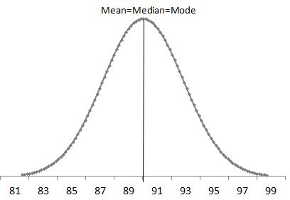
- The Mean, Median, and Mode are equal for normal distribution.
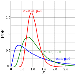
Lognormal distribution
- A continuous random variable x follows a lognormal distribution if its natural logarithm, ln(x) follows a normal distribution.
- When you sum the random variables, as the sample size increases, the sum distribution becomes a normal distribution, regardless of the distribution of the individuals. The same scenario applies to multiplication.
- The location parameter is the mean of the data set after transformation by taking the logarithm, and also the scale parameter is the standard deviation of the data set after transformation.
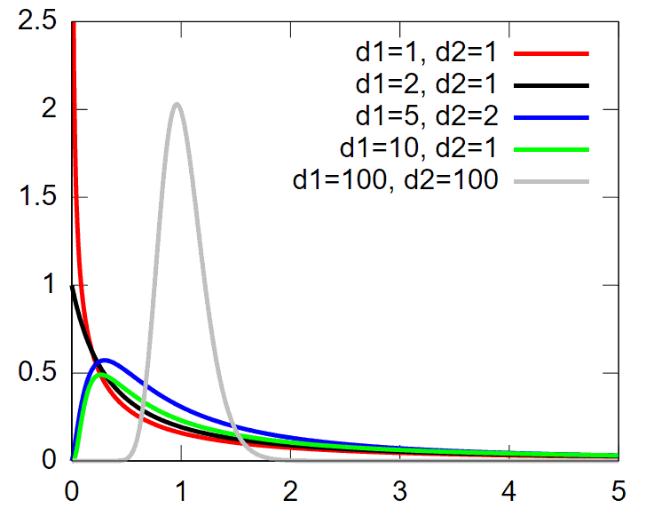
F distribution
- The F distribution extensively uses to test for equality of variances between two normal populations.
- The F distribution is an asymmetric distribution that has a minimum value of 0, but no maximum value.
- Notably, the curve approaches zero but never quite touches the horizontal axis.
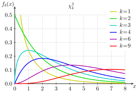
Chi Square distribution
- The chi square distribution results when independent variables with standard normal distribution are squared and summed.
- Ex: if Z is the standard normal random variable then:
- y =Z12+ Z22 +Z32 +Z42+…..+ Zn2
- The chi square distribution is symmetrical and bounded below zero. And approaches the normal distribution in shape as the degrees of freedom increase.
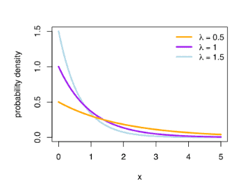
Exponential distribution
- The exponential distribution is the probability distribution of the widely used continuous distributions. Often used to model items with a constant failure rate.
- The exponential distribution is closely related to the Poisson distribution.
- Has a constant failure rate as it will always have the same shape parameters.
- Ex: The lifetime of a bulb, the time between fires in a city.
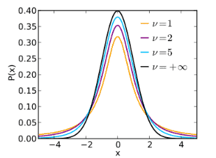
T Student distribution
- t distribution or student’s t distribution is a bell shape probability distribution, symmetrical about its mean.
- Commonly used for hypothesis testing and constructing confidence intervals for means.
- Used in place of the normal distribution when the standard deviation is unknown.
- Like the normal distribution, when random variables are averages, the average distribution tends to be normal, regardless of the distribution of the individuals.
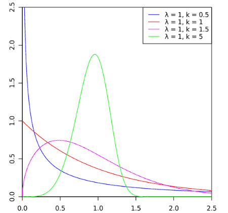
Weibull Distribution
- The basic purpose of Weibull distribution is to model time-to-failure data.
- Widely used in reliability, medical research, and statistical applications.
- Assumes many shapes depending upon the shape, scale, and location parameters. Effect of Shape parameter β on Weibull distribution:
- For instance, if shape parameter β is 1, it becomes identical to exponential distribution.
- If β is 2, then Rayleigh distribution.
- And If β between 3 and 4, then assume a Normal distribution.
Non-normal distributions
Generally, a common assumption is that while performing a hypothesis test, the data is a sample from a normal distribution, but that is not always the case. In other words, data may not follow a normal distribution. Hence, we use nonparametric tests when there is no assumption of a specific distribution for the population.
Particularly nonparametric test results are more robust against violation of the assumptions. Different types of nonparametric tests include the Sign test, Mood’s Median Test (for two samples), Mann-Whitney Test for Independent Samples, Wilcoxon Signed-Rank Test for a Single Sample, and Wilcoxon Signed-Rank Test for Paired Samples
Odd Distributions
Bivariate Distribution:
- The continuous distribution (like normal, chi square, exponential) and discrete distribution (like binomial, geometric) are the probability distribution of one random variable
- Whereas bivariate distribution is a probability of a certain event occurring in case two independent random variables exist, it may be a continuous or discrete distribution.
- Bivariate distribution is unique because it is the joint distribution of two variables.
- A bi-modal distribution has two modes. In other words, two outcomes are most likely to compare the outcomes of their region.
- 2 sources of data come into a single process screen.
How to Evaluate a Data Distribution
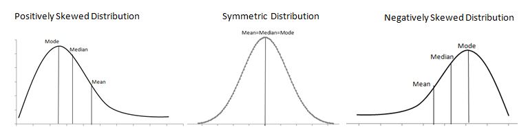
The shape of data distribution is depicted by its number of peaks and symmetry possession, skewness, or uniformity. Skewness is a measure of the lack of symmetry. In other words, skewness measures how much a random variable’s probability distribution deviates from the Normal Distribution.
We classify the skewed distribution as either left-side (a negatively skewed distribution) or right-side (a positively skewed distribution). Both sides of the mean do NOT match.
Use Graphical Analysis to show how the points are distributed and the data arranged throughout the set. These distributions graphically illustrate the data’s spread (dispersion, variability, or scatter).
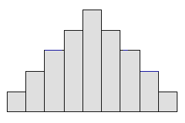
Symmetrical Distribution
Generally, symmetrical distribution appears as a bell curve. The perfect normal distribution is the probability distribution that has zero skewness. However, it is always impossible to have a perfect normal distribution in the real world, so the skewness is not equal to zero; it is almost zero. Symmetrical distribution occurs when mean, median, and mode occur at the same point, and the values of variables occur at regular frequencies. Both sides of the mean match & mirror each other.
Example: High school students weigh between 80lbs and 100lbs, and the majority of students weigh around 90lbs. The weights are equally distributed on both sides of 90 lbs, which is the center value. This type of distribution is called a Normal Distribution.
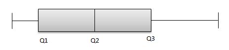
Similarly, symmetric distribution also can be reviewed with boxplot
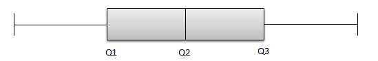
The above graph is a boxplot of symmetric distribution. The distance between Q1 & Q2 and also Q2 & Q3 is equal.
Q3-Q2 = Q2-Q1
Though the distance between Q1 & Q2 and Q2 & Q3 is equal, it is insufficient to conclude that the data follows a symmetric distribution. The team also has to look at the length of the whisker, and if the distance of the whisker is equal, then we can conclude the distribution is symmetric.
Examples of Symmetric data distributions: Normal Distribution, Uniform
Positively Skewed Distribution
We say that a distribution skews to the right if it has a long tail that trails toward the right side. The skewness value of a positively skewed distribution is greater than zero.
Example: The income details of the Chicago manufacturing employees indicate that most people earn between $20K and $50K per annum. Very few earn less than $10K, and very few earn $100K. The center value is $50K. It is very clear from the graph a long tail is on the right side of the center value.
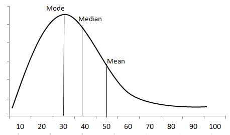
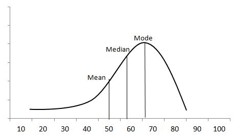
The distribution is positively skewed as the tail is on the positive side of the center value. Unlike symmetric distribution, it is not equally distributed on both sides of the center value. From the graph, it is clearly understood that the mean value is the highest one, followed by the median and mode.
Since the skewness of the distribution is towards the right, the mean is greater than the median and ultimately moves towards the right. Also, the mode of the values occurs at the highest frequency on the left side of the median. Hence, mode < median < mean.
Box plot
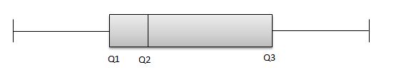
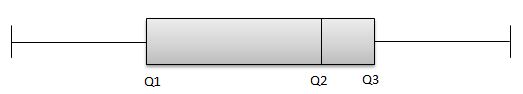
From the above boxplot, Q2 is present very near to Q1. So, it is a positive skew distribution.
Q3-Q2>Q2-Q1
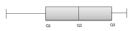
So, it clearly indicates that the data is skewness towards positive. But, for instance, if the graph is like the one below, then:
From the above picture, Q2-Q1 and Q3-Q2 are equal. But the distribution is still positive-skewed because the length of the right whisker is much greater than the left whisker. So, we can conclude that the data is positively skewed.
In summary, always check the equality of Q2-Q1 and Q3-Q2. If it is equal, check the whiskers’ length to conclude the data distribution.
Negatively Skewed Distribution
A distribution is said to be skewed to the left if it has a long tail that trails toward the left side. The skewness value of a negatively skewed distribution is less than zero.
Example: A professor collected students’ marks in a science subject. The majority of students score between 50 and 80, while the center value is 50 marks. The long tail is on the left side of the center value because it is skewed to the left-hand side of the center value. So the data is negative skew distribution.
Here mean < median < mode
From the above boxplot, Q2 is present very near to Q3. So, it is a negative skew distribution.
Q3-Q2<Q2-Q1
Similarly, like above, Q2-Q1 and Q3-Q2 are equal. But the distribution is still negatively skewed because the length of the left whisker is much greater than the right whisker. So, we can conclude that the data is negatively skewed.
It is good to transform the skewed data into normally distributed data. Data can transform using methods like Power transformation, Log transformation, and Exponential transformation.
Statistical Tests Used to Identify Data Distribution
There are different methods to test the normality of data, including visual or graphical methods and Quantifiable or numerical methods.
Visual method: A Visual inspection approach may be used to assess the data distribution normality, although this method is unpredictable and does not guarantee that the data distribution is normal. However, the visual method somewhat helps the user judge the data normality.
Ex: Histogram), boxplot, stem-and-leaf plot, probability-probability plot, and quantile-quantile plot.
Quantifiable method: Quantifiable methods are supplementary to visual methods. Particularly these tests compare the scores in the sample to a normally distributed set of scores with the same mean and standard deviation.
Ex: Anderson-Darling Test, Shapiro-Wilk W Test, Kolmogorov-Smirnov Test etc.,
Other Data Distribution Notes:
Don’t like or can’t use the existing distribution? So, a data transformation turns the data set into something more easily analyzed.
How to Make a Process Follow a Normal Distribution by Using Transforms
Sometimes you will be analyzing a process, and the data will come out in a non-normal shape. Since normal distributions have wonderful mathematical properties that make analysis and control so much easier, try to transform the data to a normal distribution if possible.
The approach to address the non-normal distribution is to make the transformation to “normalize” the data. Some typical data transformation methods are Box Cox, Log transformation, Square root or power transformation, Exponential and Reciprocal, etc.,
- A Box Cox transformation is a useful power transformation technique used to transform non-normal dependent variables into a normal shape.
- George Box and Sir D.R.Cox. are the authors of this method
- The applicable formula is yl =yλ (λ is the power or parameter to transform the data).
- For instance, λ=2, the data is squared, and if λ=0.5, then a square root is required.
- Z transformation is an analysis tool in signal processing
- It is a generalization of the Discrete-Time Fourier Transform (DTFT), in particular, it applies to signals for which DFTF doesn’t exist, thus allowing you to analyze those signals
- It also helps to see the new ideas in the sense of a system with respect to stability and causality
- Z transform is the discrete-time counterpart to the Lapse transform

Comments (8)
Hi Ted –
It appears that the above Binomial link isn’t working.
Thank you sir!
Jeff
Thanks, Jeff. It should be all set now!
Hi Ted, the link is still not working
Manish – I replaced the broken link for binomial in the article text. The one that Jeff references is still broken. I’ll remove the one from his comment.
Best, Ted
Ted,
I have been using these videos as a supplement to your material since distributions and statistics are new to me.
You might consider including them for each distribution type: https://www.youtube.com/playlist?list=PLTNMv857s9WVzutwxaMb0YZKW7hoveGLS
I’ll take a look – thanks for suggesting, Derek!
Hello
I think to really understand stats, one needs to start from raw data such as weights (quantitative cont), number of kids (quantitative discrete), marital status (qualitative) data in a real group of people and start explaining stats from there. that is describe the type of data (parametric, non-para), how to summerize dat (means, SD vs freq and proportions), how to compare groups and correlate and other tests. Also real examples on probabilities.
If this is not done then that means only one thing which is the tutor himself has no Scooby about anything in stats. Here for instance I still did not understand what is meant by probability distribution in real life.
Thank you for your thoughtful comment. Statistics becomes far more meaningful when it’s grounded in real-world data that people can relate to, like weight, number of children, or marital status. That hands-on, practical approach is exactly what we strive for at SixSigmaStudyGuide.com.
To clarify one key point: a probability distribution in real life simply describes how likely each possible value of a variable is to occur. For example, if you randomly selected people and measured their weights, a normal (bell curve) distribution might describe how those weights are spread out; with most people near the average and fewer at the extremes.
We cover this concept in detail in our article on data distributions, which includes practical examples of both discrete and continuous data, and how distributions differ depending on the data type and context. It’s also worth checking out our articles on descriptive statistics and inferential statistics to explore how to summarize and compare data effectively. From calculating means and standard deviations to choosing the right test based on whether your data is parametric or non-parametric, you should be able to find answers there.
Your suggestion — to start with raw, relatable data and build understanding from the ground up — is not only valid, it’s essential. That’s exactly the approach we take in our full courses, such as the Green Belt program, where we guide learners step-by-step through concepts with examples that mirror the real world.
If there’s a specific topic or type of data you’d like to see explained in more depth, I’d love to hear more — and happy to expand the content to make it more useful to you and others.