The one and two-sample proportion hypothesis tests involve one factor with one and two samples, and likewise, these tests may assume a binomial distribution. If more than two samples exist then use the Chi-Square test.
One Sample Z Proportion Hypothesis Test
The One Sample Proportion Test is used to estimate the proportion of a population. It compares the proportion to a target or reference value and also calculates a range of values that is likely to include the population proportion. This is also called the hypothesis of inequality.
Furthermore, use normal approximation or binomial enumeration based on the sample size. If the sample size is large, the normal approximation works well. If the sample size is small, use binomial enumeration. It is exact, so it is the safer choice for small samples.
Assumptions of the one sample Z Proportion test
Firstly, the data are random values from the population
Secondly, the population follows a binomial distribution
Null hypothesis: population proportion is equal to the hypothesized proportion
Alternative hypothesis: population proportion is not equal to or different from the hypothesized proportion (two-tailed)
Population proportion is greater than the hypothesized proportion (one-tailed)
Population proportion is less than the hypothesized proportion (one-tailed)
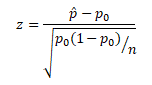
Test statistic for one sample Z proportions test
Where
z is the test statistic
p̂is
observed proportion
P0 is the hypothesized probability
n is the sample size
Procedure to execute One Sample Z Proportion Hypothesis Test
Firstly, state the null hypothesis and alternative hypothesis
State alpha, in other words, determines the significance level
Thirdly, compute the test statistic
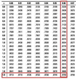
Fourthly, determine the critical value (from the critical value table)
Then, define the rejection criteria
Finally, interpret the result. In the event that the test statistic falls in the critical region, reject the null hypothesis
Example of One Sample Z Proportion Test
A researcher claims that Republican Party will win in the next Senate elections, especially in Florida State. Statistical data reported that 23% voted for Republican Party in the last election. To test the claim a researcher surveyed 80 people and found 22 said they voted for Republican Party in the last election. Is there enough evidence at α=0.05 to support this claim?
P0=0.23
n=80
p̂=22/80=0.275
Then, define the Null and Alternative hypothesis
Null Hypothesis: p= 0.23
Alternative Hypothesis: p≠0.23
State Alpha
α=0.05
State decision rule
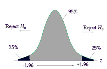
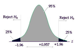
The critical value is ±1.96, hence reject the null hypothesis if the calculated value is less than -1.96 or greater than +1.96
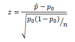
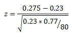
Then, calculate the test statistic
= 0.045 / 0.047 = 0.957
Each shaded tail holds 2.5% (α/2), not 25%. The middle holds 95%.
Since the calculated value is between -1.96 and 1.96 and it is not in the critical region, hence failed to reject the null hypothesis.
Six Sigma Black Belt Certification One Sample Proportion ZTest Questions:
Question: Which of the following statement is true, the right-tailed test of a single sample proportion test statistic value is +1.12 and the critical value from the table is +2.89.
(A) Reject the null hypothesis (B) Failed to reject the null hypothesis (C) Accept the null alternative hypothesis (D) None of the above
The 1 Sample Sign Non Parametric Hypothesis test was invented by Dr. Arbuthnot a Scottish physician in the year 1710. The Sign test is used to test the null hypothesis that the median of a distribution is equal to some hypothesized value k. The test is based on the direction or the data are recorded as plus and minus signs rather than numerical magnitude, hence it is called the Sign test.
Use sign test for the following:
To determine the preference for one product over the other
Conduct a test for the median of a single population (one sample sign test)
To perform a test for the median of paired difference using the data from two dependent samples.
One Sample Sign Test
The One-sample Sign Test determines a significance test of a hypothesized median value for a single data set. The 1 sample sign test is a Non Parametric Hypothesis test used to determine whether a statistically significant difference exists between the median of a non-normally distributed continuous data set and a standard. This test basically concerns the median of a continuous population.
The 1 sample sign test is to compare the total number of observations less than (-ve) or greater than (+) the hypothesized value. The 1 sample sign test is similar to the One-sample Wilcoxon Signed-rank test but less powerful than the Wilcoxon signed test.
The One-sample Sign Test is a non parametric version of one sample t-test. Similar to one sample t-test, the sign test for a population median can be a one-tailed (right or left-tailed) or two-tailed distribution based on the hypothesis.
Left tailed test- H0:median≥ Hypothesized value k; H1: median <k
Right tailed test- H0:median≤ Hypothesized value k; H1: median >k
Two-tailed test- H0: median= Hypothesized value k; H1: median ≠k
Assumptions of the one sample sign test
The data do not need to follow a normal distribution.
A random sample of independent measurements for a population with an unknown median
The variable of interest is continuous
1 sample test handles a non-symmetric data set, which means skewed either to the right or the left.
Procedure to execute One Sample Sign Non Parametric Hypothesis Test
State the claim of the test and determine the null hypothesis and alternative hypothesis
Determine the level of significance
Assign positive and negative signs to the sample data, and determine the sample size (n)- n is the sum of positive and negative signs
Find critical value
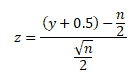
Compute the test statistic-
If n≤ 25 (approx), use y. Where y is the smaller number of positive and negative signs
For a larger sample size, if n > 25, use
Make a decision, the null hypothesis will be rejected if the test statistic is less than or equal to the critical value
Interpret the decision in the context of the original claim.
Example of One Sample Sign Test
A Bank of America West Palm Beach, FL branch manager shows that the median number of savings account customers per day is 64. A clerk from the same branch claims that it was more than 64. The clerk found the number of savings accounts customers per day data for 10 random days. Can we reject the branch manager’s claim at a 0.05 significance level?
Null Hypothesis H0: Savings account customer median = 64;
Alternative Hypothesis H1: Savings account customer median >64
Assign observations less than 64 with a – sign and observations above 64 with a + sign
Total number of + values =8
Total number of – values =2
Test statistic is a minimum of (8,2) =2
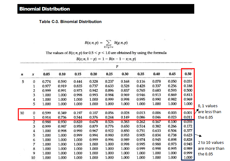
Look at the Binomial table (10, 0.5)
Note: 10- is the number of trials
0.5 – 50% chance more than the median value and 50% chance less than the median value
At 0.05 significance level
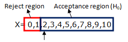
The probability of 2 or fewer minus signs, P(X ≤ 2) = 0.001 + 0.010 + 0.044 = 0.055, is greater than 0.05. Since test statistic 2 is in the acceptance region ( H0), hence failed to reject the null hypothesis. So, there is no significant evidence that the number of savings account customers per day is more than 64.
Six Sigma Black Belt Certification 1 Sample Sign Non Parametric Hypothesis Test Questions:
The preferred non-parametric method for unpaired samples is the Mann-Whitney non parametric hypothesis test or Mann-Whitney test (it is also called as Wilcoxon Rank Sum Test or the Mann-Whitney Wilcoxon Test) and thus the non parametric solution to evaluating two independent datasets comparable to the Student’s T-test.
The Mann-Whitney U test is a non-parametric statistical test used to compare two independent samples. It assesses whether the distribution of values in one sample is stochastically greater or less than the distribution of values in another sample. This test does not specifically compare sample means, but rather it evaluates whether the two samples come from the same population or if one tends to have higher values than the other.
How Decision Rules Differ Between Mann-Whitney U and Parametric t-Tests
It’s important to understand how the Mann-Whitney U test differs in decision-making from parametric tests like the independent or paired t-test. While all of these tests aim to determine if two groups differ, their approaches and interpretations are different:
Parametric t-Tests: These tests compare means and assume that the underlying data follows a normal distribution. A small p-value in a t-test typically leads to the conclusion that there is a statistically significant difference in average values between the two groups.
Mann-Whitney U Test: This test does not compare means. Instead, it ranks the data and tests whether values in one group tend to be higher or lower than those in the other group. It makes no assumption about the shape of the distribution, making it a safer option when data is skewed or ordinal. A significant p-value here suggests that one population tends to yield higher (or lower) values than the other, but not necessarily that their medians or means differ.
So, while both tests help you reject or accept a null hypothesis, the t-test focuses on differences in central tendency (mean), and the Mann-Whitney focuses on differences in rank distributions.
A few researchers also interpret the Mann-Whitney test will help to compare the medians of the two populations. Usually, parametric tests will compare the means (Null hypothesis: μ1=μ2) between the independent groups. Whereas, the null hypotheses and the two-sided hypotheses non-parametric tests can be indicated as follows:
Null Hypothesis (H₀): The two populations come from the same distribution.
Alternative Hypothesis (H₁): The two populations come from different distributions.
Note: Unlike t-tests, Mann-Whitney does not assume a difference in means, only a difference in distribution or tendency.
The Mann-Whitney test is regularly performed as a two-sided test, therefore the investigative hypothesis indicates that the two populations are not equal, instead of specifying the directionality.
Assumptions of the Mann-Whitney:
The sample drawn from the population is random.
Independence within the samples and also mutual independence is assumed. That means that an observation is in one group or in the other (it cannot be in both).
The data do not need to be normal. To read the result as a difference in medians, both distributions should have the same shape and spread.
The Mann-Whitney U test can be used in many industries, but it is most frequently applied in healthcare, nursing, business, and related fields. In medicine, it is a more efficient method to know the effect of two medicines and whether they are equal or not. It is also used to know whether or not a particular medicine cures an ailment or not.
Procedure to conduct Mann-Whitney test
Combine the two data samples into a single dataset and sort them in ascending order.
Assign ranks to all observations.
Separate the ranks back into their original groups.
Calculate the U statistic using the sum of ranks for each group.
Find the critical U value from the Mann-Whitney table based on your sample sizes and significance level.
Compare the calculated U value to the critical value and draw a conclusion.
Calculation of Mann-Whitney Test
Case 1: For comparing two small sets of observations (samples sizes less than 20)
U1 = n1n2+0.5n1(n1+1)-R1
U2 = n1n2+0.5n2(n2+1)-R2
Where
U1+U2=n1n2
n1 is the observations from the first population
n2 is the observations from the second population
R1 is the sum of observation ranks for the first population
R2 is the sum of observation ranks for the second population
Finally, calculate the U statistic as the smaller U1 and U2. U= min (U1, U2)
Case2: Normal approximation and tie correction
For sample sizes above ~20, the distribution of U rapidly approaches the normal distribution
U mean = μU =0.5 n1n2
Example of Mann-Whitney Test
A researcher, while conducting studies on the Biomass of various trees, wished to determine if there was a difference in the biomass of male and female Juniper trees. So, he randomly selected 6 individuals of each gender from the field. He dries them to constant moisture, chips them, and then weighs them to the nearest kg.
H0: There is no difference between the biomass of male and female Juniper trees– Biomassmale = Biomassfemale (medians are equal)
H1: There is a difference between the biomass of male and female Juniper trees– Biomassmale ≠ Biomassfemale (medians are not equal)
The samples are small (6 and 6) and we do not assume normal biomass, so a non-parametric test is appropriate: the Mann-Whitney U test (the non-parametric counterpart of an independent measures t-test).
Mann-Whitney Table: For Two-Tailed Test at a 5% Significance Level
Ucritical = 5
Calculated U is a value less than the critical value of U for a 0.05 significance level. Ucalculated < Ucritical . Hence, we can reject the null hypothesis.
Therefore, we reject the null hypothesis and conclude that there is a statistically significant difference in the biomass distributions between male and female Juniper trees.
Six Sigma Black Belt Certification Mann-Whitney Test Questions:
Question: Which of the following test is calculated by ranking all the participant’s scores from lowest to highest and adding up the ranks separately for each of the groups?
Six Sigma terminology, sometimes politely called “terminology” but more accurately described as jargon, can overwhelm new learners. If you are studying for a Green Belt or Black Belt, the vocabulary alone can feel like learning a new language.
One reader captured this challenge perfectly in a survey response:
“I’m studying for Green Belt and the jargon is mind blowing. I think to make this more accessible and understandable for fresh students who are not aware of LSS, the narrative needs to be diluted and the jargon made simpler. The classic example is something like the explanation of a standard distribution as the mechanism for gaining the benchmark is not very clear.” – Karle
Karle is absolutely right.
Many Six Sigma books and instructors assume you already speak the language. Terms like sigma level, process capability, control limits, and standard deviation are often introduced quickly, sometimes with little connection to real-world applications.
The result is predictable: students memorize vocabulary without understanding how it works.
This article fixes that.
Instead of repeating textbook definitions, we will explain the most common Six Sigma terms in clear language, connect them to real business problems, and show how they fit inside the broader improvement framework. If you want the more formal definitions alongside these, ASQ’s quality glossary is a solid cross-reference.
Why Six Sigma Jargon Exists
Before learning the terminology, it helps to understand why the jargon exists in the first place.
Six Sigma developed at Motorola in the 1980s as a data-driven methodology for reducing defects and improving processes. The approach draws heavily from statistics, quality engineering, and operations management.
Although jargon can be frustrating, it serves a purpose.
Standard terminology allows teams to communicate precisely.
When someone says:
“Process capability is 1.33”
Everyone in the room immediately understands the implication.
However, effective practitioners translate these terms into business language for stakeholders.
How to Learn Six Sigma Terminology Faster
Instead of memorizing definitions, try these strategies.
Connect Terms to Real Work
Relate concepts to your own processes.
Visualize the Data
Charts and graphs make statistical concepts intuitive.
Apply the Concepts
Work through small improvement projects.
Ask Questions
If terminology feels confusing, it usually means the explanation was poor, not that the concept is impossible.
A Commitment to Jargon-Free Learning
At SixSigmaStudyGuide.com, the goal is simple:
Make Six Sigma clear and practical.
There are already hundreds of jargon-free articles on the site, and more are being added regularly.
If you encounter a term that still feels confusing:
Use the search bar on the site
Read the related articles
Leave a question in the comments if anything remains unclear
Thousands of learners visit the site, and the community frequently helps answer questions.
Sometimes the fastest way to learn Six Sigma is to hear the concept explained in plain language by someone who has applied it in real life.
When you're ready, there are a few ways I can help:
First, join 12,000+ other Six Sigma professionals by subscribing to my email newsletter. A short read every Monday to start your work week off correctly. Always free.
* * *
If you're looking to pass your Six Sigma Yellow Belt, Green Belt or Black Belt exam, I'd recommend starting with my affordable study guide:
1)→ 🟡Pass Your Six Sigma Yellow Belt: built for ASQ, IASSC and ILSSI, 1,700+ practice questions with explanations, and six full-length mock exams for your exam
2)→ 🟢Pass Your Six Sigma Green Belt: a study guide organized by the exam Body of Knowledge, 1,300+ practice questions with detailed answer explanations, and 20 full-length mock exams
3)→ ⚫Pass Your Six Sigma Black Belt: the full Black Belt Body of Knowledge, 2,200+ practice questions with detailed answer explanations, and 20 full-length mock exams
You've spent so much effort learning Lean Six Sigma. Why leave passing your certification exam up to chance? This comprehensive study guide offers 1,700+ exam-like questions for Yellow Belts, 1,300+ for Green Belts and 2,200+ for Black Belts with full answer walkthroughs, access to instructors, detailed study material, and more.
The IASSC Lean Six Sigma Green Belt Study Guide is a free, quick-reference list of essential material to prepare for and pass the certification exam. Master the IASSC Six Sigma Greenbelt Body of Knowledge with this Study Guide.
When you’re ready, there are a few ways I can help:
First, join 12,000+ other Six Sigma professionals by subscribing to my email newsletter. A short read every Monday to start your work week off correctly. Always free.
* * *
If you’re looking to pass your Six Sigma Yellow Belt, Green Belt or Black Belt exam, I’d recommend starting with my affordable study guide:
1)→ 🟡Pass Your Six Sigma Yellow Belt: built for ASQ, IASSC and ILSSI, 1,700+ practice questions with explanations, and six full-length mock exams for your exam
2)→ 🟢Pass Your Six Sigma Green Belt: a study guide organized by the exam Body of Knowledge, 1,300+ practice questions with detailed answer explanations, and 20 full-length mock exams
3)→ ⚫Pass Your Six Sigma Black Belt: the full Black Belt Body of Knowledge, 2,200+ practice questions with detailed answer explanations, and 20 full-length mock exams
You’ve spent so much effort learning Lean Six Sigma. Why leave passing your certification exam up to chance? This comprehensive study guide offers 1,700+ exam-like questions for Yellow Belts, 1,300+ for Green Belts and 2,200+ for Black Belts with full answer walkthroughs, access to instructors, detailed study material, and more.