
Control Charts Study Guide

Control charts are among the hardest things to understand for those studying Six Sigma. Here’s an easy Control Charts Study Guide for you.

While studying for the Six Sigma Black Belt Exam, I noticed many questions on the control charts. Besides that, I noticed that there were a lot of different types of control charts. You had to use one for certain kinds of data or the number of units in the sample. Then you had to use other control charts in different instances.

Preparing for a Six Sigma exam? Get the I-MR Chart Worked Exercise kit.

A step-by-step Excel workbook (live formulas, Phase I baseline + Phase II monitoring + a blank template) and a printable PDF walkthrough covering the moving-range method, the Rule 1 and Rule 4 signals, and the exam angle. Enter your email and I'll send it now.

You'll also get my weekly Six Sigma newsletter. Unsubscribe anytime.

Beyond that, several of the data sets go with different distribution types. You take this for granted when a question is specifically about data. However, I found it was easy to get tripped up on the exam when it came up in control chart questions.

Very confusing, right????

So, in the spirit of continuous improvement, we made the following control charts study guide.

Control Charts Study Guide Overview

Control Chart: A control chart is one of the primary techniques of statistical process control (SPC). It plots quality characteristics measured or computed from a sample against the sample number or time. Walter Shewhart invented the control chart at Bell Labs in the 1920s.

Statistical Process Control: Statistical Process Control (SPC) is a statistical method to measure, monitor, and control a process. In other words, SPC is a quality control method that employs statistical methods to measure, monitor, and control a process.

Common Cause: A cause of variation in the process is due to chance but not assignable to any factor. It is the variation that is inherent in the process. A process under the influence of a common cause will always be stable and predictable.

Assignable Cause (“Special Cause”): You can identify and eliminate the variation in a process that is not due to chance. A process under the influence of a special cause will not be stable and predictable.

Rational Sub-Grouping: Rational sub-grouping is the process of organizing the data into groups produced under the same conditions. Rational subgroups help in the estimation process of short-term variations. Thus, rational subgrouping is the basis for operating control charts in a successful manner. These variations later help us predict the long-term variations and their control limits, depending on the type of causes for the variation (special or common).

Control Charts by Data Type Study Guide

The control chart is a graph used to study how a process changes over time. A control chart always has a central line for the average. It also has an upper line for the upper control limit and a lower line for the lower control limit. The control limits are ±3σ from the centerline.

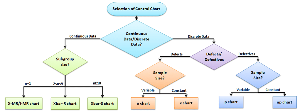
Selecting an appropriate control chart is very important in control chart mapping. Otherwise, we end up with inaccurate control limits for the data. Not all control charts are the same. Different Data Types require different charts.
Control Charts Study Guide

Control Charts for Continuous Data

Measure the output on a continuous scale. It is possible to measure the quality characteristics of a product. Once you know you are charting continuous data, determine if your population is normal or not and the sample size (n) you are charting.

No matter what you decide, I think you could start off just making a basic Run chart and seeing where that brings you. It is just a basic graph that displays data values in a time order. It can be useful for identifying trends or shifts in the process. A run chart also allows you to test for randomness in the process.

The Data is Normal

Subgroup size n = 1, then use an X-MR or I-MR chart: Use an Individual moving range (I-MR ) chart when data is continuous and not collected in subgroups. In other words, collect a single observation at a time. An I-MR chart provides process variation over time in a graphical method. 

If 1 < n < 10, then use an X bar-R chart. It monitors the process performance of continuous data collected in subgroups at set time periods. Since n is small, use the range to estimate the process variation. It consists of two plots to monitor the process mean and the process variation over time.

Else, If n >= 10, then use an X bar-S chart. It is often used to examine the process mean and standard deviation over time. Use the X bar-S chart when the subgroups have a large sample size. The S chart also gives a better understanding of the spread of subgroup data than the range.

Special Note: If your data is Not Normal

Note that there is some lively conversation in the industry on this. For your application purposes, I suggest you read the following and make your own decisions (if you’re just studying for certification, you can probably skip):

Control Charts for Discrete / Attribute Data Study Guide

Attribute control charts work with attribute data.  In other words, the data that counts the number of defective items or the number of defects per unit. For example, the number of tubes failed on a shop floor. Unlike variable charts, attribute charts plot only one chart.

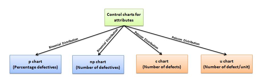
Four types of control charts exist for attribute data. P charts plot the proportion of defective items, and np charts are for the number of defectives. U charts are for the average number of defects per unit, and C charts are for the number of defects.
Control Charts Study Guide

When there are Multiple Defects (i.e., chances of being defective): It computes control limits based on the Poisson distribution.

C chart-control chart for defects. It generally monitors the number of defects in constant-size units. 

U chart-control chart for defects per unit. It generally monitors the count type of data where the sample size is greater than one. Plots the average number of defects per sample unit.

When there are NOT Multiple Defects:

This population sorts units into two piles (it’s Binomial). Samples are either good or bad, positive or negative, right or wrong.

np chart-control chart for defectives. It generally monitors the number of non-conforming or defective items in the measurement process.

p chart-control chart for proportions. It generally analyzes the proportions of non-conforming or defective items in a process.

Significance of Central Limit Theorem

The Central Limit Theorem is important for inferential statistics because it allows us to safely assume that the sampling distribution of the mean will be normal in most cases. This means that we can take advantage of statistical techniques that assume a normal distribution.

The Central Limit Theorem is one of the most profound and useful statistical and probability results. For large samples (about 30 or more), the distribution of sample means is approximately a normal distribution, whatever the population shape. The central limit theorem is vital in statistics for two main reasons: the normality assumption and the precision of the estimates.

The spread of the sample means is less (narrower) than the spread of the population you’re sampling from. With a large enough sample, the shape of the population matters less. Very skewed data needs larger samples.

  • The means of the sampling distribution of the mean is equal to the population mean µx̅ =µX
  • The standard deviation of the sample means equals the standard deviation of the population divided by the square root of the sample size: σ(x̅) = σ(x) / √(n)

Central Limit Theorem allows using confidence intervals, hypothesis testing, DOE, regression analysis, and other analytical techniques. Many statistics have approximately normal distributions for large sample sizes, even when we are sampling from a non-normal distribution.
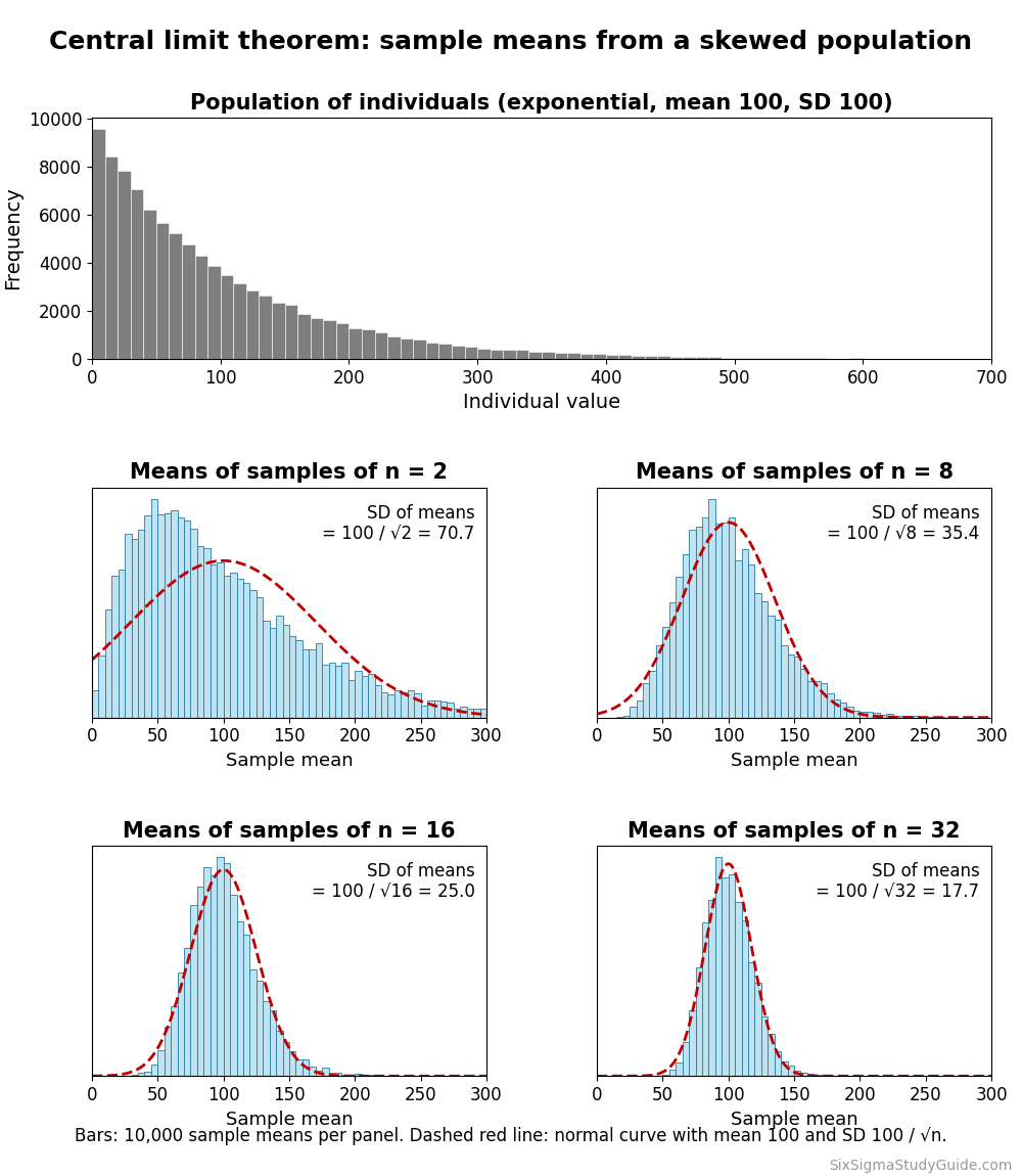
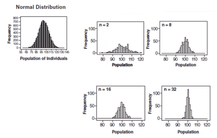
Central limit theorem demonstration: a strongly right-skewed exponential population with mean 100 and standard deviation 100, then histograms of 10,000 sample means each for n = 2, 8, 16 and 32. The means are still skewed at n = 2 and look more and more normal as n grows, centered on 100 with spread 100 divided by the square root of n (70.7, 35.4, 25.0 and 17.7).

Control charts and the central limit theorem

The analysis in the above graph uses subgroup sizes of 2, 8, 16, and 32. We can see the impact of the subgrouping. In figure 2 (n=8), the histogram is not as wide and looks more “normally” distributed than Figure 1. Figure 3 shows the histogram for subgroup averages when n = 16. It is even more narrow, and it looks more normally distributed. Figures 1 through 4 show that as n increases, the distribution becomes narrower and more bell-shaped, just as the central limit theorem says. 

This means that we can often use well-developed statistical inference procedures and probability calculations based on a normal distribution. That holds even if we are sampling from a population that is not normal, provided we have a large sample size.

Control Chart Analysis Study Guide

The main purpose of a control chart is to improve the process. It provides a “voice of the process” that helps teams to identify special causes of variation in the process. By removing the special cause from the process, the process becomes more stable and consistent.

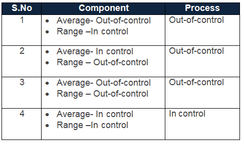
Out-of-control: A process is “out-of-control,” meaning special causes exist in either the average chart, range chart, or both. Teams must identify and eliminate special causes to achieve a stable process. We can say the process is out-of-control if any point in the control chart is out of control limits or has abnormal patterns of variability.  
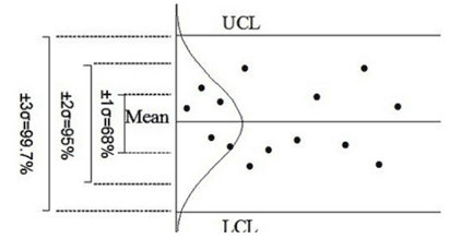
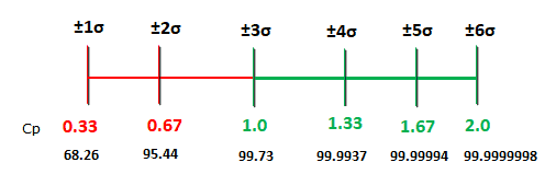
Control limits are three standard deviations above and below the mean. If the process is in control and the averages are close to normal, about 99.73% of them will fall within these limits. The range chart also uses 3 sigma limits, but ranges are not normally distributed, so its percentage is not exactly 99.73%.

Four possible conditions may occur in any process.
Control Charts Study Guide

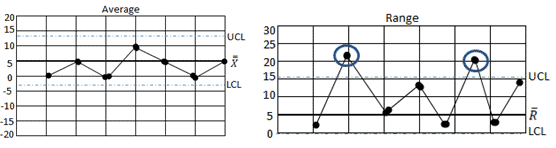
Average stable, Variation changing (Example)
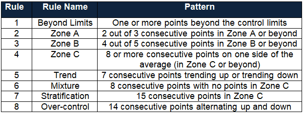
Five Common Rules for Control Chart Interpretation
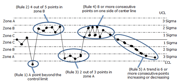
Rules 1 to 4 follow the Western Electric rules, with 8 points in a row on one side of the center line. The Nelson rules use 9 points for that run, and 6 points for a trend.

Control Chart Rules

Control Charts Study Guide Videos

Other Helpful Articles

I love MoreSteam’s visual that shows the layering of multiple tools here.

Practical Notes on Using Control Charts and Control Limits to Make Process Improvements

Practical Uses and Questions on Control Charts
Practical Uses and Questions on Control Charts. Photo by runran

Here are some Practical Notes on Using Control Charts and Control Limits to Make Process Improvements. I recently got into a great discussion on LinkedIn. Before replying to a post, I wanted to clarify my thoughts. Well, 1300 words later and a lot of digging around on forums, this is what I discovered. Hope this helps bring clarity on practical uses of Control Charts – it was a fun Sunday morning exercise!

Why should you use Control Charts to Map your Process?

Charting the process will give you the tools to verify the performance: see if a process is under statistical control. It also helps you monitor the effects of improvement efforts.

Why do you want your Process to be under Statistical Control?

Once you reach an acceptable level of stability, you can feel confident that the process will perform consistently. It is meaningless to say that the process IS 4.5 sigma if its behavior IS NOT consistent over time or is unstable.

Also, once a Process is under statistical control, you can begin to apply some of the other tools to improve performance.  Trying to improve performance before a process is under control can actually make things worse. See the Quincunx demonstration for a great visual on this.

Why you would want Control Limits less than 3 Sigma?

Control charts aim to reflect process stability, or an equivalent behavior, over time. Given a normal distribution, 99.73% of your distribution would lay inside six standard deviations or sigmas. On a control chart, half would be above and half below. Thus, positive three sigmas for the UCL – Upper Control Limit and negative three sigmas for the LCL – Lower Control Limit.

The name of the game here is to use control limits to decide if something is broken in your process. You also use them to determine if it is a special event or a common event, because that dictates your next actions. (See below).

A point outside of that Six Sigma band (above the UCL or below the LCL) means that the process is out of control. The reasoning is that a process behaving as usual is very unlikely to deliver such a point. So you could reasonably suspect that the process is no longer under control.

Too Few Sigmas

If you use control limits at too few sigmas, you are reducing the percent likelihood that a point will land in the band. Thus, you will detect any small shift in the process behavior. However, you will also have too many points outside the limits just by chance when there is no special cause to address, giving you many false alarms.

Too Many Sigmas

If you use control limits at too many sigmas, you are increasing the chances of a point landing in the bands. Virtually the whole population will fall within the limits, so there will be no false alarms. But you’ll miss most shifts in the process. That leads to missed opportunities for improvement – in which case, why are you charting the process in the first place?

The Perfect Balance

The key here is cost/risk management. We are trying to find the economic trade-off between charting the process and investigating vs. the cost of missing an instance of variation. That missed variation would cause financial issues: the cost of poor quality. Practitioners found (and widely accept) that control limits at three sigmas are a good balance.

Control limits come from historical data and process variation. As your process capability improves, you must recalculate the control limits.

When Should I Recalculate My Control Limits?

The short answer is once the control charts cease to have meaningful business applications. This could be either that you have improved or altered the original practice so much that you have, in effect, a new and different process than what you started with.

What does this look like in practice? After your process has reached a point of statistical control, you should have a good data history. Then you can begin using trend analysis.

Basic trend analysis:

  • Lack of plotted points near the control limits
  • Points avoiding the outer zones and various other out-of-control conditions.

As a result of the reduced variation in your process, the new sigma is less than the original sigma. That is, the spread of the new +/- 3 sigma limits will be less than the previous limits.

Can Control Charts tell me the Sigma Level of my Process?

Control charts do NOT measure the sigma level of an overall process. They measure whether a process is in statistical control, i.e., whether only common cause variation is present. Statistical control does not require normal data.

“3 sigma control limits” refers to stability-or equality of behavior over time. “Operating at n sigma” refers to performance.

Since +/- 3 sigma encapsulates 99.73% of the data in a normal distribution, a process with all points within the limits and no unusual patterns (runs, trends) is said to be in statistical control.

The sigma calculation is used to measure the performance or effectiveness of a process at the end of the project. Today, many industries aim for much stricter quality standards, again driven by business.

Performance is how well your process meets the specifications. Note that “specification” is not used in control charts because it has nothing to do with stability. A process operating at six sigma means that the process average is six sigmas away from the closest specification limit. That is twice as far out as the three-sigma control limits (UCL and LCL) on an individuals chart. Thus, virtually no output is out of specification.

Another way to look at this is that the process is what it is regardless of whether you chart it or not, what your control limits are, or what your graph looks like. Changing the control limits does not change your process performance and hence does not change the “sigmas” at which your process operates.

The control chart and sigma calculations are separate measurements, so always treat them that way.

What do you do if a Point falls outside the Control Limits? Ex Above the Upper Control Limit or Below the Lower Control Limit?

This depends on the history of your process.

If you are just getting started and there are points outside the limits, you must get your process under control first. Find and remove the special causes behind those points. Then recalculate the limits.

If a process was under statistical control and then you find a single point outside of the control limits, there is a special cause of variation. First, be sure this is a special, one-time-only variation. Then try to set controls in place to eliminate or prevent it from coming back. Using a prioritization tool like FMEA helps. Note that you may change your standardized process to account for the special cause variation. In that case, you’ll need to re-calculate your control limits, because you now have a new process in place.

If you find multiple points outside the control limits, special causes are present, or the process has shifted. Find and remove those causes first. Once only common cause variation remains, apply six sigma methodologies like DMAIC to reduce the variation in your process.

When you’re ready, there are a few ways I can help:

First, join 12,000+ other Six Sigma professionals by subscribing to my email newsletter. A short read every Monday to start your work week off correctly. Always free.

* * *

If you’re looking to pass your Six Sigma Yellow Belt, Green Belt or Black Belt exam, I’d recommend starting with my affordable study guide:

1)→ 🟡Pass Your Six Sigma Yellow Belt: built for ASQ, IASSC and ILSSI, 1,700+ practice questions with explanations, and six full-length mock exams for your exam

2)→ 🟢Pass Your Six Sigma Green Belt: a study guide organized by the exam Body of Knowledge, 1,300+ practice questions with detailed answer explanations, and 20 full-length mock exams

3)→ ⚫Pass Your Six Sigma Black Belt: the full Black Belt Body of Knowledge, 2,200+ practice questions with detailed answer explanations, and 20 full-length mock exams

You’ve spent so much effort learning Lean Six Sigma. Why leave passing your certification exam up to chance? This comprehensive study guide offers 1,700+ exam-like questions for Yellow Belts, 1,300+ for Green Belts and 2,200+ for Black Belts with full answer walkthroughs, access to instructors, detailed study material, and more.

​ Thousands have used this system to prepare. Join them here. 

Hypothesis Testing Overview

Overview of Hypothesis Testing
Overview of Hypothesis Testing. Photo by Hartwig HDK

You may know all the statistics in the world, but if you jump straight from those statistics to the wrong conclusion, you could make a million-dollar error. That’s where hypothesis testing comes in. It combines tried-and-tested analysis tools, real-world data, and a framework that allows us to test our assumptions and beliefs. This way, we can say how likely something is to be true or not within a given standard of accuracy.

When using hypothesis testing, we create the following:

  • A null hypothesis (H0): the assumption that the experimental results are due to chance alone; nothing (from 6M) influenced our results.
  • An alternative hypothesis (Ha): the claim that a real difference or effect exists.
null hypothesis

These hypotheses should always be mutually exclusive: if one is true, the other is false.

Once we have our null and alternative hypotheses, we evaluate them with a sample of an entire population, check our results, and conclude based on those results.

Note: We never accept a NULL hypothesis; we fail to reject it. We are always testing the NULL.

Basic Testing Process

The basic testing process consists of five steps:

  1. Identify the question
  2. Determine the significance
  3. Choose the test
  4. Interpret the results
  5. Make a decision.

Read more about the hypothesis testing process.

Terminology

This field uses a lot of specialist terminologies. We’ve collated a list of the most common terms and their meanings for easy lookup. See the hypothesis testing terminology list.

Tailed Hypothesis Tests

These tests are commonly referred to according to their ‘tails’ or the critical regions that exist within them. There are three basic types: right-tailed, left-tailed, and two-tailed. Read more about tailed hypothesis tests.

Errors in Hypothesis Testing

When discussing an error in this context, the word has a very specific meaning: it refers to rejecting a true null hypothesis (Type I error) or failing to reject a false null hypothesis (Type II error). Read more about errors in hypothesis testing.

P-Values

We use P-values to determine how statistically significant our test results are and how surprising they would be if the null hypothesis were true. A p-value is the chance of results at least this extreme when the null is true. Read more about p-values.

Types of Hypothesis Tests

One aspect of testing that can confuse the new student is finding which, out of many available tests, is correct to use.

Parametric Tests

You can use these tests when it’s implied that a distribution is assumed for the population or the data is a sample from a distribution (often a normal distribution).

Non Parametric Tests

You use non-parametric tests when you don’t know, can’t assume, and can’t identify what kind of distribution you have.

Hypothesis Test Study Guide

We run through the types of tests and briefly explain what each one is commonly used for. Read more about types of hypothesis tests.

Significance of Central Limit Theorem

The Central Limit Theorem is important for inferential statistics because it allows us to safely assume that the sampling distribution of the mean will be approximately normal for large enough samples. This means that we can take advantage of statistical techniques that assume a normal distribution.

The Central Limit Theorem is one of the most profound and useful statistical and probability results. For large samples, the sample means from any sort of distribution will follow an approximately normal distribution. A sample size of 30 is a rule of thumb; skewed data needs more. The central limit theorem is vital in statistics for two main reasons: the normality assumption and the precision of the estimates.

The spread of the sample means is less (narrower) than the spread of the population you’re sampling from. With a large enough sample, the means are near normal even when the original population is skewed.

  • The means of the sampling distribution of the mean is equal to the population mean µx̅ =µX
  • The standard deviation of the sample means equals the standard deviation of the population divided by the square root of the sample size: σ(x̅) = σ(x) / √(n)

Central Limit Theorem allows using confidence intervals, hypothesis testing, DOE, regression analysis, and other analytical techniques. Many statistics have approximately normal distributions for large sample sizes, even when we are sampling from a non-normal distribution.

Control charts and the central limit theorem

In the above graph, subgroup sizes of 2, 8, 16, and 32 were used in this analysis. We can see the impact of the subgrouping. In Figure 2 (n=8), the histogram is not as wide and looks more “normally” distributed than Figure 1. Figure 3 shows the histogram for subgroup averages when n = 16, it is even more narrow and it looks more normally distributed. Figures 1 through 4 show, that as n increases, the distribution becomes narrower and more bell-shaped -just as the central limit theorem says. This means that we can often use well-developed statistical inference procedures and probability calculations that are based on a normal distribution, even if we are sampling from a population that is not normal, provided we have a large sample size.

Overview Videos

When you’re ready, there are a few ways I can help:

First, join 12,000+ other Six Sigma professionals by subscribing to my email newsletter. A short read every Monday to start your work week off correctly. Always free.

* * *

If you’re looking to pass your Six Sigma Yellow Belt, Green Belt or Black Belt exam, I’d recommend starting with my affordable study guide:

1)→ 🟡Pass Your Six Sigma Yellow Belt: built for ASQ, IASSC and ILSSI, 1,700+ practice questions with explanations, and six full-length mock exams for your exam

2)→ 🟢Pass Your Six Sigma Green Belt: a study guide organized by the exam Body of Knowledge, 1,300+ practice questions with detailed answer explanations, and 20 full-length mock exams

3)→ ⚫Pass Your Six Sigma Black Belt: the full Black Belt Body of Knowledge, 2,200+ practice questions with detailed answer explanations, and 20 full-length mock exams

You’ve spent so much effort learning Lean Six Sigma. Why leave passing your certification exam up to chance? This comprehensive study guide offers 1,700+ exam-like questions for Yellow Belts, 1,300+ for Green Belts and 2,200+ for Black Belts with full answer walkthroughs, access to instructors, detailed study material, and more.

​ Thousands have used this system to prepare. Join them here. 

Z Score and Process Capability

Z score and Process Capability are used together to get a view of your process. The Z score or value in process capability calculation is the distance from the process mean to a specification limit (USL or LSL), measured in standard deviation units.

Z score tells the defects within the system. In other words, Z score tells the number of standard deviation existed between the mean and specification limit.

Z Score and Process Capability

How Z score impacts process capability in DMAIC project

Six Sigma method can be implemented in any industry with a five-phase structured method: DMAIC. During the measure phase, Six Sigma black belts more focus on Z Score apart from other process performances.

It is very difficult in any organization to define the defects as it varies from process to process. For example, sales, production, and finance departments, defects categories are different in all the three groups. So, it is challenging to compare the process performance. Hence, Z score plays an important role or a common platform to compare all the processes’ performance.

A higher Z score means it has more number of standard deviations within specification limits and the process average is away from the outlying limit. Whereas, lower Z value means it has less number of standard deviation. In other words, there is a variation in the output. A higher Z value means the process is more capable. It does not show that the process is stable. Check stability on a control chart first.

Benefits of Z score in DMAIC projects

  • Z score is a flexible measure to use for both variable and attribute data.
  • It helps to create the baseline for the Six Sigma projects. Also, use to assess and compare before and after process performance.
  • Z score mandates the six sigma team to define the process mean, standard deviation, specification limits for continuous data. Similarly, defects, sample size etc for attribute data.
  • Z score is a universal measurement, that can be applied for different functions within the organization like production, sales, finance, HR, administration etc.

Calculate Z score and process capability one from another

Z scores basically use them to transform a given standard distribution into something that is easy for us to calculate probabilities on. Why? So we can determine the likelihood of some event happening.

Similarly, process capability and performance that’s a measure of how centered a distribution is and how dispersed it is.

Naturally, the greater the spread, the less of a chance a process has of meeting its intended specifications.

Calculating Z value

The area outside of specification for a normal curve can be determined by Z value.

  • ZUpper =(USL-X̅)/ σ̂
  • ZLower = (X̅-LSL)/ σ̂
  • Then, Zmin = The smallest value of ZUpper and ZLower

Where

  • σ̂ is the estimate of the process standard deviation
  • and σ̂ = R̅/d2
  • X̅ is the process mean

If Zmin is negative, theX̅ is outside of the specification limit.

Zmin computed with short-term (within) sigma is a short-term Z, often written ZST.

Capability Indices

Cp is the distance between the specification limits divided by six times an estimate of the process standard deviation.

Cp =(USL-LSL)/ 6σ̂

About 99.73% of a normal distribution falls within ±3 sigma, so 6 sigma is taken as the process spread. Cp tells how many process spreads (6 sigma) fit inside the specification limits. But Cp does not take into account whether or not the process is centered. Whereas, Cpk is more useful as it considers the process centered or not.

Z Score and Process Capability

Cpk is the minimum of upper specification limit minus the current process mean. The current process mean minus lower specification limit (which gives the distance to the closest specification limit) divided by three times an estimate of the process standard deviation.

Cpk =min (USL- X̅, X̅-LSL)/ 3σ̂ = Zmin/3 = ZST/3

Hence, If you have a Z value, the equation is very easy;

Cpk = Dividing the Z score by three.

A z score is the same as a standard score; the number of standard deviations a value lies above (positive) or below (negative) the mean. Z = (X-µ)/σ

Z = x – mean of the population / standard deviation.

The issue with process capability indices is that the standard deviation estimates based on the local variation. If the process shifts or drifts over time, this short-term estimate of the process standard deviation is too small for the long term. In other words, it doesn’t reflect the long term. This will be addressed by Process performance indices.

Process performance Indices

The long term process capability indices also known as process performance indices Pp and Ppk.

Pp =(USL-LSL)/ 6s

Ppk =min (USL- X̅, X̅-LSL)/ 3s

Where s is the sample standard deviation of all the data.

Example to calculate the Cpk value using Z score

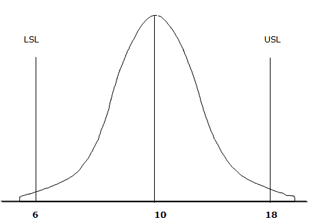
Example: The process average is 10 with an upper specification limit of 18, a lower specification limit of 6, and a standard deviation of 2. Calculate the Cpk value using Z score.

  • USL=18
  • LSL=6
  • σ̂ = 2

Now, compute ZUpper and ZLower

  • ZUpper =(USL-X̅)/ σ̂  = (18-10)/2 =4
  • ZLower =(X̅-LSL)/ σ̂ = (10-6)/2 = 2
  • So, Zmin = The smallest value of ZUpper and ZLower =2

Cpk = Zmin/3 = 2/3 = 0.667

Important Videos

When you’re ready, there are a few ways I can help:

First, join 12,000+ other Six Sigma professionals by subscribing to my email newsletter. A short read every Monday to start your work week off correctly. Always free.

* * *

If you’re looking to pass your Six Sigma Yellow Belt, Green Belt or Black Belt exam, I’d recommend starting with my affordable study guide:

1)→ 🟡Pass Your Six Sigma Yellow Belt: built for ASQ, IASSC and ILSSI, 1,700+ practice questions with explanations, and six full-length mock exams for your exam

2)→ 🟢Pass Your Six Sigma Green Belt: a study guide organized by the exam Body of Knowledge, 1,300+ practice questions with detailed answer explanations, and 20 full-length mock exams

3)→ ⚫Pass Your Six Sigma Black Belt: the full Black Belt Body of Knowledge, 2,200+ practice questions with detailed answer explanations, and 20 full-length mock exams

You’ve spent so much effort learning Lean Six Sigma. Why leave passing your certification exam up to chance? This comprehensive study guide offers 1,700+ exam-like questions for Yellow Belts, 1,300+ for Green Belts and 2,200+ for Black Belts with full answer walkthroughs, access to instructors, detailed study material, and more.

​ Thousands have used this system to prepare. Join them here. 
Z Scores and Process Sigma

Z scores and process sigma help us know what chance a process has of meeting its target. This article discusses the relation between the two concepts.

Z Scores and Process Sigma Overview

We’ve covered the basics of Z scores here. Basically, we use them to transform any normal distribution into the standard normal distribution. That makes probabilities easy to calculate. Why? So we can determine the likelihood of some event happening.

In practical applications, we often have specification limits for our process. For example, we need to create physical widgets with a length between 5 cm and 5.5 cm.  It’s important to know what the percent chance your process has of meeting that kind of target.

Assuming your process follows a normal distribution, the distance between the sample mean of your process and the upper (or lower) bound, measured in standard deviations, is the process sigma. The process sigma metric is essentially a Z equivalent.

Remember that a sigma score tells you how many standard deviations can fit between the process mean and specification limit of your process. The better your process, the more sigmas. This is a case of more is better!

When we covered the basics of Z scores, I recommended drawing a picture. That holds here, too.

Let’s look at some scenarios:

What is the Z score of a process that can NEVER meet specification?

That means you have a 100% error rate. We would be looking for an area of zero under the curve. On the chart, you’d have a negative infinity Z score.

A low sigma value means that a significant part of the process output is not inside specification limits.

What is the Z score of a process that meets specification half of the time?

If the process meets specification half of the time, the specification limit sits right at the process mean, so the Z score is 0: half of the output falls on each side. You will often see this called a 1.5 sigma process. That label comes from the sigma-level convention, which adds a 1.5 sigma shift to the long-term Z (0 + 1.5 = 1.5).

What does a low Sigma or Z score mean for your process?

A low sigma (Z) score means that your process has a lot of defects. If we made a graph of this, a significant part of the tail of the distribution extends past the specification limit.

What Z score would your process need to be at a 6 Sigma level of accuracy?

Remember, a z value counts standard deviations. The answer here is simple; a short-term Z score of 6. That is a long-term Z of 4.5 with the usual 1.5 sigma shift.

The higher the Z score, the fewer the defects there are in your process. Graphically, you would see the variation in your process  a safe distance away from the specification limit. 6 Standard deviations has been considered an industry standard as a safe distance. Some industries require greater than 6 sigma performance, though.

What Z score would reflect zero errors in the process?

This would be all of the area under the curve, or a positive infinity Z score.

How do you Calculate a Z Score from DPMO?

Ok. Let’s say you’ve calculated your baseline sigma. Let’s use the 333,333 DPMO we calculated in the example on the baseline sigma page. That’s a ratio we can express as 0.3333.

This page uses a cumulative z table: each value is the area to the left of z. If your handbook’s table shows the area from the mean (0 to z), look up 0.5 – 0.3333 = 0.1667 instead and make the z negative, since that area sits below the mean.

If you look at the Z Score table, you’ll see that 0.3333 falls between a Z score of -0.43 and -0.44 (because of the 0.3336 and 0.3300). It is very close to 0.3336, so we can say that a DPMO of 333,333 translates to a Z score of about -0.43.

When you’re ready, there are a few ways I can help:

First, join 12,000+ other Six Sigma professionals by subscribing to my email newsletter. A short read every Monday to start your work week off correctly. Always free.

* * *

If you’re looking to pass your Six Sigma Yellow Belt, Green Belt or Black Belt exam, I’d recommend starting with my affordable study guide:

1)→ 🟡Pass Your Six Sigma Yellow Belt: built for ASQ, IASSC and ILSSI, 1,700+ practice questions with explanations, and six full-length mock exams for your exam

2)→ 🟢Pass Your Six Sigma Green Belt: a study guide organized by the exam Body of Knowledge, 1,300+ practice questions with detailed answer explanations, and 20 full-length mock exams

3)→ ⚫Pass Your Six Sigma Black Belt: the full Black Belt Body of Knowledge, 2,200+ practice questions with detailed answer explanations, and 20 full-length mock exams

You’ve spent so much effort learning Lean Six Sigma. Why leave passing your certification exam up to chance? This comprehensive study guide offers 1,700+ exam-like questions for Yellow Belts, 1,300+ for Green Belts and 2,200+ for Black Belts with full answer walkthroughs, access to instructors, detailed study material, and more.

​ Thousands have used this system to prepare. Join them here. 
Measure Phase (DMAIC)

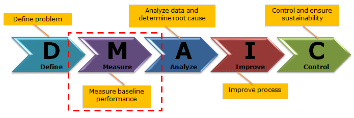
The Measure is the second phase of DMAIC. The main activity in the Measure phase is to define the baseline. While we have identified a project in the Define phase of DMAIC, let’s take the lessons learned from the first phase and get the ‘real story’ behind the current state by gathering data and interpreting what the current process is capable of.

“Life moves pretty fast. If you don’t stop and look around once in a while, you could miss it.” – Matthew Broderick as Ferris Bueller, Ferris Bueller’s Day Off. 

In the Measure phase, the Six Sigma team checks how the process is performing against the customer expectations, and CTQs are noticed in the Define phase of DMAIC.

Six Sigma Phases

Six Sigma is a systematic problem-solving approach centered around defect elimination and variation reduction, leading to process improvement.

One of the principal tools in Six Sigma is the use of the DMAIC methodology. (Also see DMAIC Overview). Particularly, DMAIC is a logical framework that helps you think through and plan improvements to a process to achieve a Six Sigma level of excellence.

There are five phases that are used in the DMAIC method.

Measure Phase (DMAIC)

The purpose of the Measure phase is to understand the extent of the problem with the help of data. In other words, measure the process performance in its current state in order to understand the problem.

Goals of Measure Phase

  • Establish baseline performance of the process
  • Identification of process performance indicators
  • Develop a data collection plan and then collect data.
  • Validating the measurement system
  • Determine the process capability

Measure Phase of DMAIC Overview

The Measure phase is approximately 2 to 3 weeks process based on the project inputs. In particular, all the relevant stakeholders’ involvement is key to getting quality data.

The measure phase is about the baseline of the current process, data collection, validating the measurement system, and determining the process capability. Multiple tools and concepts are available in the Measure phase of Six Sigma.

Process Definition & Basic Tools

Process map: A process map is a tool that graphically shows the inputs, actions, and also outputs of a process in a clear, step-by-step map of the process. 

The process map illustrates the relationship between inputs (X) and outputs (Y). Firstly, create a process map of all the activities required to convert raw materials into output (Y). Then, identify the Critical to Quality (CTQ) factors in the process.

Process map helps to identify the inefficiencies or wastes in the process. This also helps to determine the critical steps to collect the data.

Value stream mapping: Value stream mapping provides a visual representation of the organization’s flow of materials and information. A value stream map shows all the value-added and non-value-added activities needed to make the product. It consists of the process flows starting from the raw materials to making the product finally available in the hands of the customers.

Spaghetti Diagram: The spaghetti diagram, also known as the spaghetti chart, represents the basic flow of people, products, and process documents or papers.

Cause and Effect Matrix: The cause and effect matrix establishes the correlation between process input variables to the customer’s outputs during root cause analysis.

Data Collection

In fact, the measure phase is all about collecting as much data as possible to get the actual picture of the problem. Hence, the team must ensure the data collection measurement process is accurate and precise.

Data Types

Data is a set of values of qualitative or quantitative variables. It may be numbers, measurements, observations, or even just descriptions of things. Below are the types of Quantitative Data

  • Discrete data: The data is discrete if the measurements are integers or counts. For example, the number of customer complaints, weekly defects data, etc.
  • Continuous data: The data is continuous if the measurement takes on any value, usually within some range, for example, Stack height, distance, cycle time, etc.

Coding Data

Sometimes it is more efficient to code data by adding, subtracting, multiplying, or dividing by a factor.

Types of Data Coding

  • Substitution: ex. Replace 1/8ths of an inch with integer deviations from the center (for example, +1 or -1 for one eighth of an inch above or below).
  • Truncation: ex. Data set of 0.5541, 0.5542, 0.5547, you might just remove the 0.554 portions.

Data Collection Plan

A data collection plan is a useful tool to focus your data collection efforts on. This directed approach helps to avoid locating & measuring data just for the sake of doing so.

  • Identify data collection goals
  • Develop operational definitions
  • Create a sampling plan
  • Select & validate data collection methods

Plan for and begin collecting data

  • Data collection form: In general, a data collection form is a way of recording the approach to obtaining the data that need to perform the analysis. Additionally, the data should be recorded by trained operators with a calibrated instrument and a standard data collection form.
  • Data Collection check sheets: A Check Sheet is a data collection tool that usually identifies where and how often problems appear in a product or service. It’s specifically designed for the kind of process being investigated. 

Measurement System Analysis

Measurement System Analysis (MSA) is an experimental and mathematical method of determining how much variation within the measurement process contributes to overall process variability.

Accuracy: It is the difference between the true average and the observed average. If the average value differs from the true average, this is an indication of an inaccurate system.

Precision: Precision refers to how close the data points fall in relation to each other. In other words, a high-precision process will have little variance between the individual measurement points.

Gage R&R

The Gage Repeatability and Reproducibility is a method to assess the measurement system’s repeatability and reproducibility. Furthermore, Gage R&R measures the amount of variability in measurements caused by the measurement system itself.

Gage R&R focuses on two key aspects of measurement:

Repeatability: Repeatability is the variation between successive measurements of the same part, same characteristic, by the same person using the same gage.

Reproducibility: Reproducibility is the difference in the average of the measurements made by different people using the same instrument when measuring the identical characteristic on the same part.

Six Sigma Statistics

Basic Six Sigma statistics is the foundation for Six Sigma projects. It allows us to numerically describe the data that characterizes the process Xs and Ys. 

Statistics is the science of gathering, classifying, arranging, analyzing, interpreting, and presenting numerical data to make inferences about the population from the sample drawn. There are two main branches: descriptive statistics and inferential statistics.

Inferential statistics: It uses a sample to draw conclusions about the population.

Descriptive statistics: A descriptive statistic is basically organizing and summarizing the data using numbers and graphs. Descriptive statistics is to describe the characteristics of the sample or population.

The shape of data distribution is depicted by its number of peaks and symmetry possession, skewness, or uniformity. Skewness is a measure of the lack of symmetry. A normal distribution has zero skewness, but so does any other symmetric distribution. Positive skew means a longer right tail. Negative skew means a longer left tail.

Data Organization / Data Display / Data Patterns

The graphical analysis creates pictures of the data, which will help to understand the patterns and also the correlation between process parameters. Moreover, graphical analysis is the starting point for any problem-solving method. Hence select the right tool to identify the data patterns and display the data.

  • Control Chart: The control chart is a graphical display of quality characteristics that have been measured or computed from a sample versus the sample number or time.
  • Frequency Plots: Frequency plots allow you to summarize lots of data in a graphical manner making it easy to see the distribution of that data and process capability, especially when compared to specifications.
  • Box Plot: A box plot is a pictorial representation of continuous data. In other words, the Box plot shows the maximum, minimum, median, interquartile range Q1, Q3, and outlier.
  • Main Effects plot: The main effects plot is the simplest graphical tool to determine the relative impact of various inputs on the output of interest.
  • Histogram: Histogram is the graphical representation of a frequency distribution. In fact, it is in the form of a rectangle with class intervals as bases and the corresponding frequencies as heights.
  • Scatter plot: A Scatter Analysis is used when you need to compare two data sets against each other to determine a relationship.
  • Pareto Chart: Pareto chart is a graphical tool to map and grade business process problems from the most recurrent to the least frequent.

Basic Probability & Hypothesis tests

Basic Six Sigma Probability terms like independence, mutually exclusive, compound events, and more are the necessary foundations for statistical analysis.

Additive law: Additive law is the probability of the union of two events. There are two scenarios in additive law:

  • When events are not mutually exclusive
  • When events are mutually exclusive

Multiplication law: It is a method to find the probability of events occurring simultaneously. There are two scenarios in multiplication law:

  • When events are independent
  • When events are dependent

Compound Event: It is an event that has more than one possible outcome of an experiment. In other words, compound events are composed of two or more events.

Independent Event: Events can be independent events when the outcome of one event does not influence another event’s outcome. 

Hypothesis Testing

Hypothesis testing is a key procedure in inferential statistics used to make statistical decisions using experimental data. It is basically an assumption that we make about the population parameter.

When using hypothesis testing, we create:

  • A null hypothesis (H0): the assumption that the experimental results are due to chance alone; nothing (from 6M) influenced our results.
  • An alternative hypothesis (Ha): we expect to find a particular outcome.

Determine the process capability

Process Capability Analysis tells us how well a process meets a set of specification limits based on a sample of data taken from a process. The process capability study helps to establish the process baseline and measure the future state performance. Revisit the operational definitions and specify what are defects and which are opportunities.

Calculate the baseline process sigma

The value in making a sigma calculation is that it abstracts your level of quality enough so that you can compare levels of quality across different fields (and different distributions.) In other words, the sigma value (or even DPMO) is a universal metric that can help you with the industry benchmark/competitors.

Baseline Sigma for discrete data

Calculate the process capability through the number of defects per opportunity. The acceptable number to achieve Six Sigma is 3.4 Defects Per Million Opportunities (DPMO).

  • DPO = Defects/(Units * Opportunity)
  • DPMO = Defects / (Units * Opportunities) * 1,000,000
  • Yield = 1 – DPO. This is the share of opportunities with no defect. The share of whole units with no defect is about e-DPU, where DPU is defects per unit. That is lower when a unit has many opportunities.

Baseline Sigma for Continuous data

Process Capability is the determination of the adequacy of the process concerning the customer needs. Process capability compares the output of an in-control process to the specification limits.  Cp and Cpk are considered short-term potential capability measures for a process.

Cpk shows how far the process mean is from the nearest specification limit, measured in units of three standard deviations. The same distance counted in single standard deviations is Z min, which equals 3 x Cpk. 

  • Cplower = (Process Mean – LSL)/(3*Standard Deviation)
  • Cpupper = (USL – Process Mean)/(3*Standard Deviation)
  • Cpk is the smallest value of the Cpl or Cpu:  Cpk= Min (Cpl, Cpu)

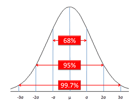
Six Sigma derives from the normal or bell curve in statistics, where each interval indicates one sigma or one standard deviation. Moreover, Sigma is a statistical term that refers to the standard deviation of a process about its mean. In a normally distributed process, 99.73% of measurement will fall within ±3σ, and 99.99932% will fall within ±4.5σ.

Measure Phase of DMAIC Deliverables

  • Detailed process map
  • Data collection plan and collected data
  • Results of Measurement system analysis
  • Graphical analysis of data
  • Process capability and sigma baseline

Measure Phase of DMAIC Videos

When you’re ready, there are a few ways I can help:

First, join 12,000+ other Six Sigma professionals by subscribing to my email newsletter. A short read every Monday to start your work week off correctly. Always free.

* * *

If you’re looking to pass your Six Sigma Yellow Belt, Green Belt or Black Belt exam, I’d recommend starting with my affordable study guide:

1)→ 🟡Pass Your Six Sigma Yellow Belt: built for ASQ, IASSC and ILSSI, 1,700+ practice questions with explanations, and six full-length mock exams for your exam

2)→ 🟢Pass Your Six Sigma Green Belt: a study guide organized by the exam Body of Knowledge, 1,300+ practice questions with detailed answer explanations, and 20 full-length mock exams

3)→ ⚫Pass Your Six Sigma Black Belt: the full Black Belt Body of Knowledge, 2,200+ practice questions with detailed answer explanations, and 20 full-length mock exams

You’ve spent so much effort learning Lean Six Sigma. Why leave passing your certification exam up to chance? This comprehensive study guide offers 1,700+ exam-like questions for Yellow Belts, 1,300+ for Green Belts and 2,200+ for Black Belts with full answer walkthroughs, access to instructors, detailed study material, and more.

​ Thousands have used this system to prepare. Join them here.