The 1 Sample Sign Non Parametric Hypothesis test was invented by Dr. Arbuthnot a Scottish physician in the year 1710. The Sign test is used to test the null hypothesis that the median of a distribution is equal to some hypothesized value k. The test is based on the direction or the data are recorded as plus and minus signs rather than numerical magnitude, hence it is called the Sign test.
Use sign test for the following:
To determine the preference for one product over the other
Conduct a test for the median of a single population (one sample sign test)
To perform a test for the median of paired difference using the data from two dependent samples.
One Sample Sign Test
The One-sample Sign Test determines a significance test of a hypothesized median value for a single data set. The 1 sample sign test is a Non Parametric Hypothesis test used to determine whether a statistically significant difference exists between the median of a non-normally distributed continuous data set and a standard. This test basically concerns the median of a continuous population.
The 1 sample sign test is to compare the total number of observations less than (-ve) or greater than (+) the hypothesized value. The 1 sample sign test is similar to the One-sample Wilcoxon Signed-rank test but less powerful than the Wilcoxon signed test.
The One-sample Sign Test is a non parametric version of one sample t-test. Similar to one sample t-test, the sign test for a population median can be a one-tailed (right or left-tailed) or two-tailed distribution based on the hypothesis.
Left tailed test- H0:median≥ Hypothesized value k; H1: median <k
Right tailed test- H0:median≤ Hypothesized value k; H1: median >k
Two-tailed test- H0: median= Hypothesized value k; H1: median ≠k
Assumptions of the one sample sign test
Data is non-normally distributed.
A random sample of independent measurements for a population with an unknown median
The variable of interest is continuous
1 sample test handles a non-symmetric data set, which means skewed either to the right or the left.
Procedure to execute One Sample Sign Non Parametric Hypothesis Test
State the claim of the test and determine the null hypothesis and alternative hypothesis
Determine the level of significance
Assign positive and negative signs to the sample data, and determine the sample size (n)- n is the sum of positive and negative signs
Find critical value
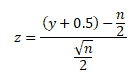
Compute the test statistic-
If n≤ 25 (approx), use y. Where y is the smaller number of positive and negative signs
For a larger sample size, if n > 25, use
Make a decision, the null hypothesis will be rejected if the test statistic is less than or equal to the critical value
Interpret the decision in the context of the original claim.
Example of One Sample Sign Test
A Bank of America West Palm Beach, FL branch manager shows that the median number of savings account customers per day is 64. A clerk from the same branch claims that it was more than 64. The clerk found the number of savings accounts customers per day data for 10 random days. Can we reject the branch manager’s claim at a 0.05 significance level?
Null Hypothesis H0: Savings account customer median = 64;
Alternative Hypothesis H1: Savings account customer median >64
Assign observations less than 64 with a – sign and observations above 64 with a + sign
Total number of + values =8
Total number of – values =2
Test statistic is a minimum of (8,2) =2
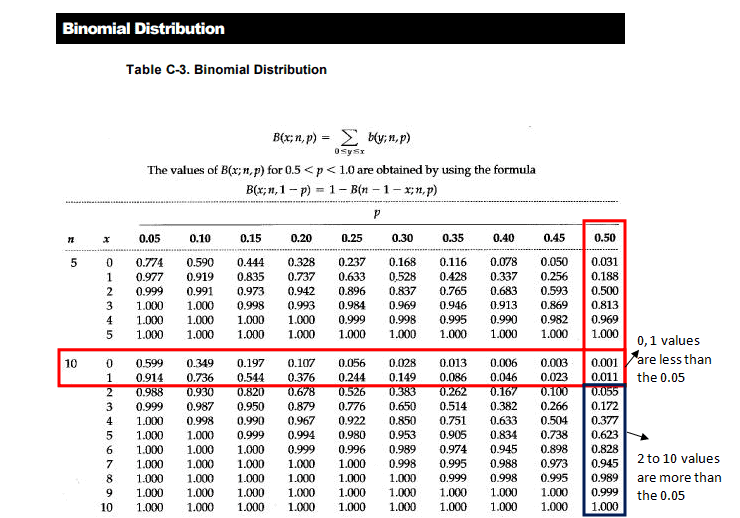
Look at the Binomial table (10, 0.5)
Note: 10- is the number of trails
0.5 – 50% chance more than the median value and 50% change less than the median value
At 0.05 significance level
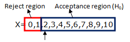
The probability for x=2 is 0.055, which is greater than 0.05. Since test statistic 2 is in the acceptance region ( H0), hence failed to reject the null hypothesis. So, there is no significant evidence that the number of savings account customers per day is more than 64.
Six Sigma Black Belt Certification 1 Sample Sign Non Parametric Hypothesis Test Questions:
The Friedman Non Parametric hypothesis test is an alternative to the one-way ANOVA with repeated measures. The Friedman Test was developed by the American economist Milton Friedman in the 1930s as a non-parametric alternative to repeated measures ANOVA. His foundational work includes publications from 1937, 1939, and 1940 that formalized ranking-based analysis across matched groups.
The Friedman Non Parametric hypothesis test is to test for differences between groups (three or more paired groups) when the dependent variable is at least ordinal. Friedman test is preferred when compared to other non parametric tests in a situation where the same parameter has been measured under different conditions on the same subject. Example: Patient Serum content monitoring before treatment, after one month, and after three months of treatment.
Friedman’s test is similar to the Kruskal-Wallis Test and also an extension of the sign test. This test is the best statistic to use for a repeated measures type of experiment to determine if a particular factor also has an effect.
The Friedman test is designed to test whether the k paired samples (k>2) of n size, are from the same population or the samples from populations having similar properties, considering the position parameter.
While the Friedman Test is robust and non-parametric, it’s important to note that it generally has less statistical power than parametric methods like repeated measures ANOVA, especially when parametric assumptions are met. This means it may be less likely to detect actual differences when they exist.
Assumptions of the Friedman Test
The group is a random sample from the population
No interaction between blocks (rows) and treatment levels (columns)
The one group that is measured on three or more different occasions
Data should be at least an ordinal or continuous
The samples do not need to be normally distributed
Procedure to conduct Friedman Test
Rank each row (block) together and independently of the other rows. When there are ties, the average ranks of the observations.
Sum the ranks for each column (treatments) and then sum the squared columns’ total
The Friedman statistic can be approximated by a chi-square distribution with (k – 1) degrees of freedom when the sample size is large enough. A common guideline is that n should be greater than 15, or the number of treatments (k) should be greater than 4, for the approximation to be reliable. For smaller datasets, exact critical values should be used instead.
Formulate decision and conclusion
Calculation of Friedman Non Parametric Hypothesis Test
The test
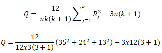
statics of Friedman’s test is
where Rj is the sum of the ranks for sample j.
n is the
number of independent blocks
k is the
number of groups or treatment levels
DF= number of groups -1 (k-1)
Null Hypotheses H0: Median treatment effects of the population are all the same
Alternative Hypotheses H1: There is a difference in treatment effects.
If the Friedman test indicates a statistically significant difference, it does not tell you which groups differ. To determine this, post-hoc tests such as the Nemenyi or Conover tests should be applied to perform pairwise comparisons.
Example of Friedman Non Parametric Hypothesis Test
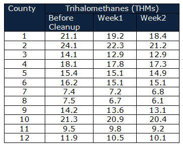
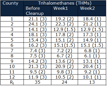
Department of Public health and safety monitors whether the measures taken to clean up drinking water were effective. Trihalomethanes (THMs) in 12 counties drinking water compared before cleanup, 1 week later, and 2 weeks after cleanup.
Null
Hypothesis H0 = the cleanup system had no effect on the THMs
Alternative
Hypothesis H1= the cleanup system effected the THMs
Significance
level α=0.05
Calculate
the Rj
Q=20.16
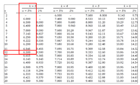
For the values of independent blocks (n) greater than 20 and/or values of groups (k) greater than 6, use χ2 table with k-1 degrees of freedom otherwise use the Friedman table
The calculated Q value is greater than the critical value of Q for a 0.05 significance level. Qcalculated >Qcritical hence reject the null hypotheses.
So, it is concluded
that the cleanup system effected the THMs of drinking water
Six Sigma Black Belt Certification Friedman Non Parametric Test Questions:
Question: A psychologist monitored the same group of students’ reactions while watching comic films and compared the students’ reactions when watching political and drama films. The tabulated data is skewed. Which of the following test to be used to analyze the data?
When you’re ready, there are a few ways I can help:
First, join 12,000+ other Six Sigma professionals by subscribing to my email newsletter. A short read every Monday to start your work week off correctly. Always free.
* * *
If you’re looking to pass your Six Sigma Green Belt or Black Belt exams, I’d recommend starting with my affordable study guide:
1)→ 🟢Pass Your Six Sigma Green Belt: a study guide organized by the exam Body of Knowledge, 1,000+ practice questions with detailed answer explanations, and 8 full-length mock exams
2)→ ⚫Pass Your Six Sigma Black Belt: the full Black Belt Body of Knowledge, 2,000+ practice questions with detailed answer explanations, and 8 full-length mock exams
You’ve spent so much effort learning Lean Six Sigma. Why leave passing your certification exam up to chance? This comprehensive study guide offers 1,000+ exam-like questions for Green Belts (2,000+ for Black Belts) with full answer walkthroughs, access to instructors, detailed study material, and more.
The Kruskal–Wallis Non Parametric Hypothesis Test (1952) is a nonparametric analog of the one-way analysis of variance. It is generally used when the measurement variable does not meet the normality assumptions of one-way ANOVA. It is also a popular nonparametric test to compare outcomes among three or more independent (unmatched) groups.
Consider the Mann-Whitney test for just two groups instead of the Kruskal-Wallis test. Like the Mann-Whitney test, this test may also evaluate the differences between the groups by estimating the differences in ranks among the groups.
Generally in the ANOVA test, the assumption is that the dependent variable is drawn from a normally distributed population and also assumes that common variance across groups. But, in Kruskal-Wallis Test, there is no necessity for these assumptions. Therefore, this test is the best option for both continuous as well as ordinal types of data.
Assumptions of the Kruskal-Wallis Test
All samples are randomly drawn from their respective population.
Note: This test evaluates differences in mean ranks and that interpreting these differences as differences in medians requires the assumption of similarly shaped distributions across groups. If you’re not comparing similarly shaped distributions, the test may detect differences due to those inconsistent shapes rather than the differences between the central tendencies.
Uses of Kruskal-Wallis Non Parametric Hypothesis Test Test
The Kruskal-Wallis test can be used for any industry to understand the dependent variable when it has three or more independent groups. For example, this test helps to understand the student’s performance in exams. While the scores are measured on a scale from 0-100, the scores may vary based on the exam anxiety levels (low, medium, high, and severe -in this case, four different groups) of the students.
Procedure to conduct Kruskal-Wallis Test
First pool all the data across the groups.
Rank the data from 1 for the smallest value of the dependent variable and the next smallest variable rank 2 and so on… (if any value ties, in that case, it is advised to use mid-point), N being the highest variable.
This reliance on ranks can make the Kruskal-Wallis test less powerful than a one-way ANOVA, especially when the assumptions of ANOVA are met.
Calculation of the Kruskal-Wallis Non Parametric Hypothesis Test
The Kruskal–Wallis Non Parametric Hypothesis Test compares differences in mean ranks among k groups (k > 2). Interpreting these differences as differences in medians requires the assumption of similarly shaped distributions across the groups.
The null and alternative hypotheses for the Kruskal-Wallis test are as follows:
Null
Hypothesis H0: Population medians are equal
Alternative
Hypothesis H1: Population medians are not all equal
As explained above, the procedure for the Kruskal-Wallis test pools the observations from the k groups into one combined sample, and then ranks from lowest to highest value (1 to N), where N is the total number of values in all the groups.
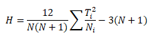
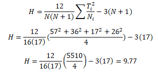
The test statistic for the Kruskal Wallis test (mostly denoted as H) is defined as follows:
Where Ti = rank sum for the
ith sample i = 1, 2,…,k
The Kruskal-Wallis test is more robust to outliers than parametric tests because it operates on ranked data rather than raw values. As a result, extreme values (high or low) tend to have less impact on the test statistic. However, in smaller datasets, even a few extreme values can still shift the rank distribution enough to influence the results, especially if those outliers affect the relative ordering between groups.
Note on Sample Sizes:
The Kruskal-Wallis test is a non-parametric alternative to one-way ANOVA and relies on ranks rather than raw values. While it doesn’t assume normality, it does require sufficient sample size for reliable results, especially when interpreting the approximate chi-square distribution of the test statistic.
To ensure validity:
Minimum per group: Aim for at least 5 observations per group, but:
Prefer 10+ per group for more stable and reliable p-values.
20+ per group is ideal when possible, especially with tied ranks or unequal variances.
Minimum number of groups: The test requires at least 3 groups to test for differences in medians.
Avoid small group sizes with ties or skewed data: The chi-square approximation becomes unreliable with:
Heavily tied data
Unequal group sizes, especially when some groups are small
Small samples (<5 per group):
The p-value may be inaccurate under the chi-square approximation.
In such cases, consider using exact p-values or Monte Carlo simulations (some statistical packages support this).
Rule of Thumb Summary
Sample Size per Group
Validity of Chi-Square Approximation
< 5
Not recommended
5-9
Acceptable but borderline
10-19
Generally reliable
≥ 20
Strongly recommended for robustness
Important Note on Interpretation:
While many texts describe the Kruskal-Wallis test as comparing group medians, this is only strictly valid if the distributions across groups are similarly shaped and scaled. In practice, the test detects differences in the distribution of ranks, which can result from differences in location (medians), spread (variability), or shape. Technically, the Kruskal-Wallis test is a test of stochastic dominance, not median equality. That means it’s possible to have equal medians across groups and still reject the null hypothesis if other aspects of the distributions differ. Always inspect distribution shapes before interpreting results solely in terms of medians.
Example of Kruskal-Wallis Non Parametric Hypothesis Test
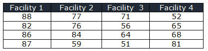
In a manufacturing unit, four teams of operators were randomly selected and sent to four different facilities for machining techniques training. After the training, the supervisor conducted the exam and recorded the test scores. At 95% confidence level does the scores are same in all four facilities?
Null Hypothesis H0: The distribution of operator scores are same
Alternative Hypothesis H1: The scores may vary in four facilities
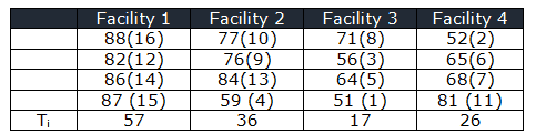
Rank the score in all the facilities
N=16
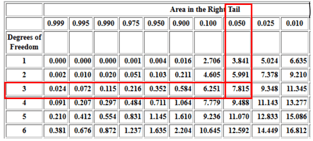
While for a right-tailed chi-square test with a 95% confidence level, and df =3, the critical χ2 value is 7.81
Critical values of Chi-Square Distribution
The calculated χ2 value is greater than the critical value of χ2for a 0.05 significance level. χ2calculated >χ2critical hence, you reject the null hypotheses
So, there is enough evidence to conclude that difference in test scores exists for four teaching methods at different facilities.
Six Sigma Black Belt Certification Kruskal-Wallis Test Questions:
Question 1: In an organization, management conducted a study comparing Purchase, Marketing, Quality, and Production groups on a measure of leadership skills. Which of the following test would an organization choose?
When you’re ready, there are a few ways I can help:
First, join 12,000+ other Six Sigma professionals by subscribing to my email newsletter. A short read every Monday to start your work week off correctly. Always free.
* * *
If you’re looking to pass your Six Sigma Green Belt or Black Belt exams, I’d recommend starting with my affordable study guide:
1)→ 🟢Pass Your Six Sigma Green Belt: a study guide organized by the exam Body of Knowledge, 1,000+ practice questions with detailed answer explanations, and 8 full-length mock exams
2)→ ⚫Pass Your Six Sigma Black Belt: the full Black Belt Body of Knowledge, 2,000+ practice questions with detailed answer explanations, and 8 full-length mock exams
You’ve spent so much effort learning Lean Six Sigma. Why leave passing your certification exam up to chance? This comprehensive study guide offers 1,000+ exam-like questions for Green Belts (2,000+ for Black Belts) with full answer walkthroughs, access to instructors, detailed study material, and more.
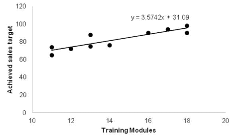
A Regression Analysis gauges the relationships between different variables by looking at the behavior of the system. Many analysis techniques can show the relationship between dependent and independent variables. However, a Regression Analysis is one of the best. For example, you can use transformations to reduce the higher-order terms in the model.
Remember the equation for a line that you learned in high school? Y = mx + b. Here, m is the slope of the line, and b is the point on the y-axis where the line intercepts. Given m and b, you can plug in any value for X and get a result y. Very simple and very useful. That’s what we are trying to do in root cause analysis when we say “solve for y.”
Though people describe statistical linear models as a classic straight line, linear models often show up as curvilinear graphs. Non-linear regression, aka Attributes Data Analysis, explains the nonlinear relationship between a response variable and one or more predictor variables (mostly a curved line).
Unfortunately, real life systems do not always boil down to a simple math problem. Sometimes you just have a collection of points on a graph. Then your boss tells you to make sense of them. That’s where regression analysis comes into play. You are basically trying to derive an equation from the graph of your data.
“In the business world, the rear view mirror is always clearer than the windshield.”
Warren Buffett
Linear Regression Analysis
The easiest kind of regression is linear regression. Imagine that all of your data falls in a neat row. If you could draw a straight line through all the points, that line would model the simple equation Y = mx + b from earlier. That would give you a model that would predict what your system would do given any input of x.
The Method of least squares creates the best possible approximation of a line for the data set.
To see how well the line fits the data, use the Standard Error of Estimate. The larger the Standard Error of the Estimate, the greater the distance of the charted points from the line.
The normal rules of Standard Deviation apply here. So 68% of the points should be within +/- 1 Standard Error of the line, and 95.5% within +/- 2 Standard Error.
Just take the square root of the Coefficient of Determination, Sqrt(R Squared). Then give it the same sign as the slope. A line that slopes down has a negative r.
Use the F statistic to find a p-value of the system. The degrees of freedom for the regression equal the number of Xs in the equation. For example, in a linear regression analysis this is 1, because there is only 1 x in y=mx+b.
Null Hypothesis: Suggests that there is no statistical significance between the two variables in the study.
Alternative Hypothesis: Suggests that there is statistical significance between the two variables in the study.
The smaller the p-value, the better. But really, you judge this by finding the acceptable level of alpha risk. Then you check if that % is greater than the p-value. Alpha is that false-alarm risk. An alpha of 0.05 means that when no real relationship exists, 5% of the time we will falsely reject the null hypothesis and conclude there is one. The p-value is different. It is the probability of seeing a relationship at least this strong in the sample if there were none.
For example, say your alpha risk level is 5% and the p-value is 0.014. Then we can reject the null hypothesis and may conclude that there exists a relationship between the variables. In this case, you’d accept the line because there is a significant relationship between the variables.
Additional Helpful Resources
Looking for something more advanced than what’s on the exam? See Canonical Correlation Analysis. It is a multivariate technique for relating two whole sets of variables to each other at once, and it goes beyond the official Green Belt/Black Belt Body of Knowledge.
Residual Analysis: “Since a linear regression model is not always appropriate for the data, assess the appropriateness of the model by defining residuals and examining residual plots.”
What is the difference between Residual Analysis and Regression Analysis?
Regression models, a residual measures how far away a point is from the regression line.In a residual analysis, residuals are used to assess the validity of a statistical or ML model. The model is considered a good fit if the residuals are randomly distributed.
The third guest post in a series from Jeremy Garret.
In my first article I explained how Lean Six Sigma literally saved my teaching career, and shared a few general insights into how Lean Six Sigma can be used in other careers. Manufacturing, computer programming, and more recently even human resources have used Lean Six Sigma and other related quality assurance systems to increase efficiency, decrease product or process failures, save time, save money, and even increase profit. The public school systems in the United States are in desperate need of those same improvements.
Budget cuts are pressuring schools to accomplish more with less funds at the same time that changes in technology are rapidly raising the minimum education needed to get a good, stable job. Broad unemployment and international competition are further pressuring U.S. schools to improve. Unfortunately state and local leaders are seldom trained in the use of quality assurance systems such as Lean Six Sigma. Even if a principal or superintendent was trained in Lean Six Sigma support would be needed from both above and below within the rest of the school administration. While introducing Lean Six Sigma to state departments of education would almost certainly produce tremendous benefits, we don’t have to wait. Individuals can (and should) apply the fundamental skills of Lean Six Sigma within their own careers.
Studying and applying the principles of Lean Six Sigma has indeed changed my life and my career! During my studies of Lean Six Sigma I learned that my own teaching methods could be treated much like a manufacturing process, that I could continuously tweak my teaching and grading processes by using a scientific analysis of my students’ grades and behaviors. Prior to that realization, my instructional plans were far too rigid and I was too eager to blame my students and our government. In short, I was bad and unhappy. Changing my perspective and a few of my behaviors has made me a happier and more successful teacher; it is that path to success that I want to continue to share with you in this post.
Here is a quote from my immediate supervisor (our math department head) describing the changes from her point of view:
Our department would not be the same without you in it! I have seen the change in your classroom over the years and it is definitely better for you and the students.
In my second post I explained how control charts displaying class grade averages on the vertical axis (or “y-axis”) and time on the horizontal axis (or “x-axis”) allowed me to see with great detail when I needed to: 1) reteach a subject, 2) change my grading on an assignment, or 3) both. That level of information and my response to it greatly decreased the number of parent conferences and greatly improved the ones that remained. The change in parent conferences combined with other improvements greatly improved how my supervisors thought of me and how they reviewed my performance. The techniques discussed in this and other posts can be used in a great many settings; it is my belief that you too can apply these techniques in your job or in your life. If you have already used such techniques or intend to do so, please help us by sharing your experiences with us (by using the comment section below).
Unfortunately the level of information provided by the basic control charts was not enough to tell how grading systems should be modified, such charts only indicated when modifications are needed. In order to determine how grading should best be done (or redone) I had to know what the distribution of the grades was and when those distributions changed. I measured the change in the distributions by using a type of control chart that showed a class’s standard deviation on the vertical axis and time on the horizontal axis. I could tell when special problems had arisen by looking for times at which a class’s standard deviation was different from the others or when it had suddenly changed. To gain a deep insight into situation I then used a histogram that showed how many students earned each letter grade (A, B, C, etc). In this article I will show the types of special problems that the standard deviation control chart (or “S chart”) can find. I will explain how histograms showed the severity and nature of the problems that had been found by the control chart. I will conclude by explaining how I used that information to create “fair, data-driven, scientific grading curves.”
Basic Control Charts
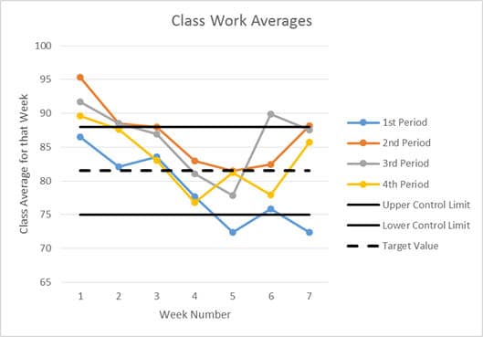
Before demonstrating the standard deviation control chart, I want to pause for just a moment to show you the “regular” class average control that was discussed in the previous article. (As stated in previous articles, all of the data shown in these graphs come from actually classes that I taught during the 2013-14 school year and represent actual problems that I faced and addressed using these techniques.)
class work averages
In this chart, the upper and lower control limits were created using a combination of personal experience and feedback from administrators. In manufacturing these limits would normally be set by calculating three times the standard deviation that was observed during initial testing; in both cases, these control limits must be well within the user specification limits (which are generally not shown on a control chart). The dotted line shows the target value; it is nearly always just an average of the two control limits.
In this chart we can see that three of four classes had an average that was “too high” during week one. It also shows that 1st Period had grades that were clearly “too low” for two weeks and borderline “too low” during one more. This also shows that something unusual seems to have happened to the 3rd Period class during week six.
Standard Deviation Control Charts
In spite of the power of that chart, we are still unable to tell what caused the changes. Additional information can be gained by looking at the standard deviations of the classes’ classwork averages. These standard deviations can tell us how spread out the individual student’s grades were from each other. Given that our data is actually classwork grades, we should expect to have at least one student with a 100% and at least one at or near a 0%, thus the class-wide range would not be particularly useful. The standard deviation however can tell us if the “weak students” are performing only a little below the “strong students” (a small standard deviation) or if the performance of the two groups is dramatically different (a large standard deviation). It should be noted that “a little below” and “dramatically different” must be determined by the teacher’s experience; in industry however there are very precise tables and equations for calculating these values.
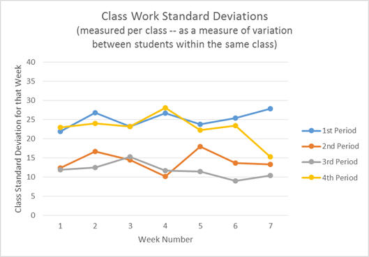
Creating a control chart with the class period standard deviations (measuring the variance between students within each class) produced the following chart.
class work standard deviations
(Technically, this is a “run chart” instead of a “control chart” since no control limits have been added to the graph.)
The first thing that most people notice from this graph is that 1st and 4th period consistently had a larger standard deviation than 2nd and 3rd period. This means that the grades were more spread out in 1st and 4th than they were in 2nd and 3rd. We can also see that during week seven 4th period had a drop in the spread of the grades.
At this point in an analysis it is very tempting to guess at a cause and move on. With experience and intuition many people can correctly identify at least one valid cause of the variation (in this case the spread of the grades), but even the most seasoned quality professionals cannot guess all of the causes immediately and even they cannot immediately guess which cause is the most important. So it is important to keep an open mind and not guess — not yet. (Guessing at a solution without adequate data is one of the biggest reasons for the large inefficiencies found in the U.S. education system.) In this situation, a histogram can tell us a LOT more about our students, their needs, and what options might help them the most.
Comparisons to Graphs Used in Industry
Before moving further, it is important to compare the analyses that we’ve done so far to those used in industry. The first two types of charts that we made form a set called “X-bar and S,” where “X-bar” is an abbreviation for the average of a set of measurements and “S” is an abbreviation for standard deviation. It should be noted however that the “X-bar and S” charts that we have created are different from the most commonly used types in a very important way. In manufacturing “X-Bar” normally indicates measurements that were averaged over time, for example you might take a measurement every few seconds and then average the last 20 data points. Similarly, “S” would thus be a standard deviation of those last twenty measurements.
In our graphs we averaged across twenty to thirty students who completed tasks all at the same time; this is equivalent to measuring multiple machines running at the same time. This type of analysis is also commonly used in industry to compare employees and machines that were all running at the same time, but it is important to be aware that this is different from what is normally meant by the term “X-bar and S” graphs. The most important difference is the type of information revealed. The more common type of “X-bar and S” graphs could be used to measure day to day changes for each student; as a teacher I feel that I can capture this information more easily using qualitative data (which I will cover in a later post). In contrast, my concern is the class period to class period differences and the differences in overall grades from one day to the next, both of which will be revealed with the types of analysis being demonstrated in this post.
Histograms
A histogram chart can be generated on individual assignments (individual processes in industry) or on aggregate data such as semester or course grades. Over the last ten years of teaching I have had three different administrators require me and my fellow teachers to analyze our exam grades and semester grades by using histograms. Due to the high value of the information generated I recommend (and even beg) that histograms be used on all nine-week overall grades and on all uniquely important grades (such as final exams).
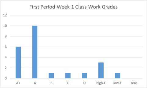
In the following example, the grades for 1st period class work from week 1 has been used. There are plugins for MS Excel that make the creation of histograms quick to generate, and there are many other programs can also be used. Without a plugin or advanced program, counting the number of grades in each category (or letter grade) is fairly quick and easy.
class histogram
Several things can be seen quite quickly from this graph. First, the grades do not have a “normal” or “bell curve” distribution or even a Rayleigh distribution. Instead the grades are clustered in the A’s and A+’s with no meaningful “tail” in the B’s & C’s, bell curve and Rayleigh distributions both gradually decrease rather than immediately dropping to almost zero. Furthermore we see a second small grouping of grades centered in the high-F range. This data shows a “bi-modal” distribution.
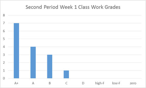
class histogram 2
In the chart above the grades from 2nd Period were used. Please remember that in the standard deviation control chart we saw that second period had a much smaller standard deviation than 1st Period. By comparing the histograms we can see a great deal of additional information. In 2nd Period the grades are all grouped around the A’s, with a significant number of students earning grades over 100%. Unlike 1st Period’s graph, this graph does show a “tail” (gradually decreasing numbers) as we move to the right (toward the lower grades). Experienced teachers can already guess which of these two classes had the fewest discipline problems and other problems, but even with accurate intuition it is important to wait to guess at the causes.
Applications and Grading Techniques
Although the standard deviation control charts are more abstract than simple average grade control charts they are correspondingly more powerful. The main reasons why is that the standard deviation is actually more sensitive to the types of problems that I am most concerned with. I have found that my strongest students perform well even on days when I, the teacher, do not. This can result from the strongest students already knowing the material or from their ability to learn it quickly in a wider range of environments.
In contrast however, I find that my weaker students are much more effected by both my performance and the type of content being taught. The weaker students are more easily distracted than the stronger students. Additionally, when the teacher is not “entertaining enough” or not providing strong classroom management then the weaker students will be off task sooner and longer than the stronger students. The weaker students also need more and better examples. Thus the weaker students will be more negatively impacted by a presentation that only has a few bad examples and only a few “you try” problems (class work problems with immediate feedback). As a result, days or weeks in which the instruction and/or classroom management are bad, the class average will drop some — but only a little, because the strong students will still have high grades. The standard deviation however will increase dramatically in these situations, because the standard deviation is a measure of the spread of the data. Thus the standard deviation chart can point to days in which weak students and strong students performed at close to the same level and when they performed at very different levels. When combined with other data (primarily qualitative, observational data) this can show when the teacher needs to focus more on classroom management, increasing the number of examples, or finding a way to be more “entertaining.”
Furthermore, since the standard deviation is an indication of the spread of the data it partially indicates the type of “curve” that is best at different times. For important grades (such as 9-week grades or a final exam), I always use a histogram to fully understand the needs of the students. For less critical situations (like a unit test or a quiz) I use the following guidelines — if the standard deviation is “small” and the average is “low” then a simple “shift” (adding a few points) is a good technique, but when the standard deviation is “high” and the average is “low” then a slightly more complicated approach is nearly always better. In these situations I have been using (and teaching my fellow teachers to use) this procedure: multiply the grades by a number slightly below one (typically 0.9 to 0.8) and then add a number that both compensates for that multiplication and that provides a small additional shift (typically 10% to 30%). For example, on most of my tests I configured my gradebook software (“INOW”) to multiply by 0.8 and to then add 30%. This techniques takes a grade of 10% and turns it into a 38% while taking a 100% and turning it into a 110%.
It should be noted that each of these benefits has its own equivalent in manufacturing and other industries. A decreased need for final product checks, a decreased need for expensive product and process audits, and a strong reputation can all result. As practical examples, Craftsman tools cost more than online generic tools, but many people (including myself) buy the more expensive ones whenever possible. Other people feel the same way about Sony and Toyota. In fact, Toyota is famous for the “Toyota Production System” or the “Toyota Method” which is built upon and contains the techniques in this article (along with many techniques not yet covered). General Electric is also famous for Six Sigma which also includes the techniques described in this (and future) chapters.
Conclusion
As demonstrated, the quantitative tools used in the quality assurance industry to improve tasks in manufacturing can be transferred to nearly any industry. Kindergarten through 12th grade education is currently suffering from cuts in funding while simultaneously being pressured to increase the amount of results. “No Child Left Behind,” increased need for high education, and even the need for more thoroughly literate “unskilled” workers have all added to the demand for increased scores on standardized tests. The combination of decreased funding and increased pressure for output produces a need for dramatic improvements in efficiency and in the quality of the schools’ internal processes. As we have seen in other industries (such as the automotive, electronic, and now software development industries) such changes are possible, practical, and even profitable! It is now time for the education industry to follow the examples set by other industries! In each of those successful industries the principles used within Lean Six Sigma have been the key. To complete the kind of transformation that our schools need and that our children deserve, Lean Six Sigma (or another quality assurance system) needs to be applied at both the state and local levels with involvement and leadership coming from state departments of education. But individual teachers and principals do not have to wait and hope for these changes. They can begin making some of these changes within their own classrooms.
One of the major components of successful quality assurance work is the correct use of control charts and histograms. In the case of K-12 education teachers can and should use these techniques to identify times when material should be retaught and times when grades should be “curved.” Doing so does involve an initial investment of time, but doing so creates a reputation for high quality teaching and fair grading in addition to the actual improvement in the curriculum and knowledge transfer. In today’s education market with law suits, private schools, vouchers, and school transfers, a school’s reputation does affect that school’s budget, further increasing the need for immediate improvements.
In my next post, I will explain how “root-cause analysis” using “fishbone diagrams” (also called Ishikawa diagrams) form the foundation of Lean Six Sigma (and other quality assurance systems) by empowering people to find the “real” or most important cause of a problem. Root-cause analysis is thus one of the most important tools for anyone to know! Please join our discussion on this and other upcoming topics.
The techniques shown in this post (and my other posts) are not limited to manufacturing or to teaching. They can be even be used in our daily lives. If you have a story or experience with such techniques, please help us by telling us your story (by using the comment section below). Similarly please let me know if you have questions. If you like what you see or have a topic that you would like to read more about, then please let us know that too.