
(TSF #27) Lean Six Sigma Case Study: Reducing Hospital Room Turnaround Time

Many new Lean Six Sigma practitioners ask what a real project looks like in practice, especially in a healthcare setting. One of our SixSigmaStudyGuide.com students, Harpreet, recently shared a success story about improving hospital room turnaround times. Let’s take a look at her project and then explore how we might enhance it using a structured Six Sigma approach.

Harpreet’s Write-Up:

Background: I work in a rural community hospital who has seen increase in emergency department volumes and admissions from ED.

We also seen increase in ALC patients (ALC patients are the patients who no longer require acute care and are awaiting in hospital bed to be discharged to an appropriate destination) blocking beds. Our hospital has 35 surgical beds, 15 medical beds and 4 ICU beds. Total of 54 beds.

Problem: The tension of improving time to admitted patient length of stay has resulted in a blame problem which in my eye is a gap in process and clarity. It was often mentioned that housekeeping department hold the beds by not promptly cleaning it. Whereas housekeeping folks complained that they are not informed in timely manner or in advance about the discharges.

I also found that we do all the process by paper. There is no electronic way to track. We don’t have white boards. Staff was not taking staggered breaks resulting in periods when housekeeping staff was unavailable.

What I did: I started tracking room turn around times. I completed the process map, collected data. I completed fishbone diagram

What Changes I made: I educated housekeeping staff about the bed issues and how it is connected to performance. Staggered breaks to better coverage. Reviewed staffing

What I found: Reduction in mean time after tracking room turn around time”

First, congratulations to Harpreet on achieving a significant reduction in mean room turnaround time! Cutting the average room turnover from ~60 minutes to ~45 minutes is a big win. It means patients can be admitted sooner and the hospital can accommodate more patients overall. This kind of result has a direct impact on patient flow and satisfaction.

Project Approach: DMAIC or Quick Improvement?

First, congratulations to Harpreet! By applying Lean Six Sigma principles, she successfully reduced mean room turnaround times, an achievement that directly improves patient access and care. Helping a rural hospital better serve its community is a powerful application of continuous improvement.

Although this project leans heavily into Lean thinking by focusing on process clarity, waste reduction, and flow, it still fits well within the DMAIC framework. Harpreet defined the problem, measured the process, analyzed the causes using tools like a fishbone diagram, implemented changes, and observed measurable improvements. In the sections below, we’ll walk through how to structure this project even more formally, enhancing its impact and making it a potential model for future improvement efforts.

What follows are not criticisms. Harpreet is already doing fantastic work! These are suggestions to extract even more value from the work she has already begun

Define: Clarify the Problem and Goal

In the Define phase, we want to clearly articulate the problem, scope, and goals. Harpreet described the issue generally; slow room turnover causing admission delays and the improvement achieved.

Defining a clear, measurable problem and tightly scoped goal gives the team clarity and prevents confusion. It also enables alignment with leadership. To enhance this, we should write a formal Problem Statement and Goal Statement.

  • Problem Statement: What is the pain point, in specific and measurable terms? For example (using hypothetical numbers): “Inpatient rooms are taking too long to turn over. Currently, the average turnaround time is 60 minutes (from patient discharge to room ready). This delays new patient admissions, causing an ER backlog and potential diversion of ~5 patients/week.”
    • This statement defines the gap between current performance and desired performance, and it links to impact (patients waiting). A great problem statement avoids jumping to causes or solutions. It quantifies the issue and why it matter
  • Goal Statement: What specific result are we targeting? Harpreet achieved ~45 minutes; perhaps the goal was “Reduce average room turnaround time from 60 to 45 minutes (a 25% reduction) within 3 months, to enable timely admissions and serve more patients per day.”
    • Setting a SMART goal (Specific, Measurable, Achievable, Relevant, Time-bound) gives the team a clear target.

Why make these edits? A well-defined problem and goal align the team and stakeholders. It ensures everyone understands the gap to close (15 minutes improvement) and the benefit of closing it (e.g. more patients admitted, less ER backlog). Defining the project boundaries (which hospital unit, which process steps) also prevents scope creep.

According to Six Sigma best practices, the problem statement should quantify the current vs. desired state and avoid implying a particular cause or blame. In this example, we focus on the turnaround time metric and the downstream effect on admissions, without yet proposing how to fix it or who is at fault.

Risks if not addressed: Without a clear problem and goal, the project might wander or stakeholders might misunderstand its purpose. For instance, if we didn’t specify the current 60-minute baseline, one person might think 50 minutes is “good enough” while another expects 30 minutes. If we didn’t tie the problem to the impact on admissions, hospital leadership might not realize why this project is critical.

Lack of clarity can lead to solving the wrong problem or failing to recognize success. Skipping this step could result in misalignment and reduced support for the project.

Measure: Capture Baseline Performance

Once the project is defined, the next step is Measure. This means collecting data on the current process.

Lean Six Sigma projects depend on understanding performance quantitatively. Establishing baseline metrics allows teams to measure the effect of their changes.

Current Strength: Harpreet has already started tracking room turnaround times.

Suggestions:

  • Translate the process to a function: Y= f(x)
  • Primary Outcome Metric (Y): Mean room turnaround time (from discharge to room-ready)
  • Supporting Process Metrics (Xs):
    • Time from discharge to housekeeping notification
    • Time from notification to cleaning start
    • Cleaning duration
  • Balancing Metric: Staff availability or coverage during peak hours

Risk of not making this change: Without these metrics, it’s hard to validate sustained improvement or identify whether further process issues remain hidden.

Additional Measure Phase Improvements

In my hypothetical numbers from the problem statement, Inoted the average was ~60 minutes, which is a great start. We can add more rigor by looking at the distribution and validity of the data:
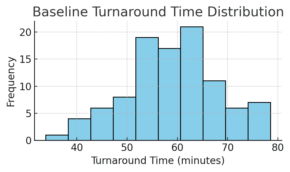
Figure: Baseline turnaround time distribution for patient rooms. This histogram shows the variation in room turnover times, with some rooms turned over in about 40 minutes, but some taking 70+ minutes. The average is around 60 minutes. Understanding the spread (min, max, common values) is as important as the mean.

  • Data Collection: How was turnaround time measured? It’s important to define the start and end points of the metric (e.g. “from patient discharge in the system to room marked clean and ready”). In one other hospital project, the team found inconsistent recording. For example, some staff recorded the end time differently, skewing the data.
    • Ensuring a consistent definition and measurement method (perhaps even doing a measurement system check) prevents garbage-in-garbage-out. For example, if half the staff weren’t stopping the clock until much later, the “60 minutes” figure might be inaccurate. We’d fix that early by training staff or automating timestamps.
  • Baseline Metrics: In addition to the mean of 60 minutes, calculate other stats: median, range, standard deviation. How much variation is there day-to-day or room-to-room? Perhaps 25% of turnarounds are taking 80+ minutes (outliers), which is crucial information. Plotting a run chart or control chart of turnaround times over several weeks could reveal patterns (maybe certain shifts or times of day are slower).
  • Process Mapping: It can help to map the process (e.g. patient discharge -> cleaning -> inspection -> ready). This isn’t about numbers but understanding each step and who is involved (nurses, transport, housekeeping). Harpreet did some of this by identifying coordination between nursing and housekeeping as an issue. A simple process map or SIPOC can ensure we consider all contributors to turnaround time.

Why emphasize Measure? Because decisions should be based on data. Baseline data is the foundation against which we’ll compare improvements. It tells us how big the problem really is and helps quantify the opportunity (e.g. “if we save 15 minutes per room, with 10 discharges a day, that’s 150 minutes saved, which is enough time to admit 3 more patients daily”).

Also, measuring variation highlights if the issue is consistent or sporadic. For instance, we might discover the median was 55 minutes but a few extreme delays pulled the average to 60, This could mean the problem might be a small number of very long turnovers. The Measure phase can also reveal root cause clues (like if nights are slower than days, etc.).

As one similar Six Sigma healthcare case study notes, “the baseline is important to compare with the improved results… Pinning down data collection early is essential for good decision-making and reliable data.” If we measure properly, we can later prove the improvement with confidence.

Risks if not addressed: If baseline data is not reliable or fully understood, the team might implement fixes that don’t actually move the needle or might miss the real problem. For example, if we didn’t catch inconsistent time logging, we might celebrate a “drop” to 45 minutes that was partly just a change in how times are recorded (a false improvement). Or we might average 60 minutes overall but fail to see that certain wards are 80+ minutes; our project might then ignore a specific bottleneck.

Skipping thorough measurement can lead to improvement efforts that are off-target or impossible to verify. We wouldn’t know for sure if we achieved success or if the process is statistically stable. Measuring poorly is like flying blind; you might land somewhere, but not necessarily at the intended destination.

Analyze: Identify Root Causes

Identify Remaining Waste and Barriers

Why: Lean aims to eliminate waste: anything that doesn’t add value to the customer (or patient, in this case). Identifying waste types can highlight hidden inefficiencies.

Suggestions:

  • Waiting: Delay between discharge and housekeeping notification
  • Motion: Manual paperwork creating unnecessary travel or effort
  • Underutilized Talent: Staff unaware of how their role impacts flow

Risk of not making this change: Hidden inefficiencies can offset the gains already achieved, and the process may not improve further without addressing them.

With baseline data in hand, the Analyze phase digs into why the turnaround time was 60 minutes. Harpreet identified coordination issues between nursing and housekeeping; let’s broaden the analysis to be sure we find all major causes:

  • Brainstorm Potential Causes: A classic tool here is the Cause-and-Effect (Fishbone) Diagram. Get the team (nurses, EVS cleaners, bed managers, etc.) together to list all factors that could slow down room turnover. Common categories to consider are People, Process, Equipment, Environment, Materials, Methods (Sometimes stated as the 6 M’s). For example, People might include staffing levels or training, Process might include unclear procedures or communication flows, Equipment could be availability of cleaning supplies or bed trackers, and so on.
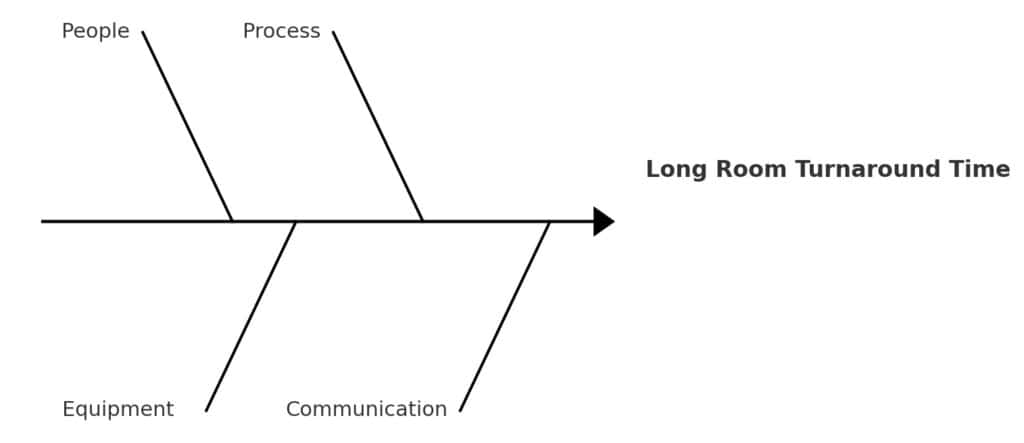
Figure: A simplified Fishbone Diagram for “Long Room Turnaround Time.” Major cause categories (people, process, equipment, communication) branch into specific issues. For instance, under People: insufficient housekeeping staff or nurses not notifying promptly; under Process: no standard protocol for “STAT” room cleaning; under Communication: delays in notifying EVS that room is ready to clean.

In Harpreet’s case, some root causes might have been:

  • No formal STAT process: Perhaps housekeeping didn’t know when a discharge was high-priority. (Like it was in this case study)
  • Communication gaps: The nurse might have marked the patient out in the system, but cleaners weren’t alerted immediately or had to be paged manually.
  • Staffing or roles: Maybe at certain times, no dedicated housekeeping staff were on standby, causing waits.
  • Standard work: Without a checklist or defined roles, cleaning could be inconsistent or slower than necessary (e.g. missing equipment, having to fetch supplies).
  • Other factors: If transportation of patients or equipment (e.g. bed cleaning machines) is involved, delays there would add to turnaround.

Harpreet did implement a checklist and better coordination, which suggests these causes were at play.

During Analyze, tools like the fishbone and even a Pareto chart can help prioritize causes. For example, if we gathered data on reasons for delays (waiting for housekeeping, room not fully cleaned, waiting for maintenance, etc.), a Pareto chart might show that two causes account for 80% of the delay (say, housekeeping response time and waiting for transport). In an OR turnover case study, “hundreds of variables may impact turnover, so the team used a fishbone diagram to prioritize the most critical factors,” identifying that equipment and attendant availability were two major contributors. We would do similarly for room turns.

  • Validate Causes: Wherever possible, back up cause hypotheses with data. If we think staffing is an issue, look at peak discharge times vs. housekeeping staffing levels. Eg Was there a spike at noon but only one cleaner on duty? If communication is a suspect, maybe logs show an average 15-minute gap from discharge to housekeeping dispatch. In other words, use process data or even observations to confirm that these factors are causing delay.

Why perform Analyze thoroughly? Because we want to fix root causes, not symptoms. It’s easy to jump to one solution (e.g., “just add more cleaners”) without realizing there’s a procedural fix (like using an automated alert to cleaners) that might be cheaper and equally effective. The analyze phase forces us to systematically consider and verify causes. Often, teams start with assumptions about the problem. Analyze helps challenge those assumptions. For instance, nurses might initially blame housekeeping, while housekeeping might blame late patient transport; analysis can reveal that both are issues, but communication is the bigger problem.

Risks if not addressed: If we skip deep analysis, we risk implementing solutions that don’t actually address the main delay drivers. Imagine if Harpreet had assumed the only issue was “housekeeping is slow” and just told them to hurry up? She might have missed that housekeeping wasn’t even notified promptly when patients left. The result could be little to no improvement, or a temporary band-aid that doesn’t last. Another risk is that without team input in analysis, you miss front-line insights and fail to get buy-in for solutions. Bypassing Analyze can also cause over-engineering: fixing things that aren’t really broken while neglecting the real bottleneck. not finding the true root causes means the improvements may only scratch the surface or target the wrong problem, and the original issue (slow turnarounds) will persist.

Improve: Implement and Validate Solutions

Prioritize Next-Level Changes

Why: Harpreet has already implemented several good changes. Further structured improvements can help lock in those gains and reduce variation.

Suggestions:

  • Implement visual controls (e.g. whiteboards or printed status trackers) to improve communication
  • Formalize standard work between discharge and cleaning
  • Continue optimizing staggered breaks using peak demand data

Risk of not making this change: Improvements might plateau. If processes aren’t standardized, performance can vary between shifts or individuals.

During Improve, we design and implement changes to address the root causes identified. Harpreet already took action by coordinating between departments and using a checklist. These are excellent solutions. Here’s how we can maximize the Improvement phase:

  • Develop Solution Ideas: Brainstorm multiple countermeasures for each major root cause. For example, if communication delay is a cause, solutions could include an automatic notification system (when nurse marks patient out, housekeeping gets an alert on their phone), or a direct phone/radio call process for STAT cleans. If lack of standard process is a cause, solutions might include a detailed Room Turnover Checklist (which Harpreet did) and training staff on it. If staffing at peak times is an issue, maybe adjust housekeeping schedules or have “float” staff. List all feasible ideas and then select the best ones based on impact and ease of implementation.
  • Pilot and Implement: It’s wise to test changes on a small scale first. Perhaps start the new procedure on one hospital floor or shift for a week, gather feedback and timing data, then roll out hospital-wide. Harpreet’s introduction of a checklist could be piloted in one ward to ensure it indeed covers all tasks and is user-friendly. Similarly, a new communication protocol can be trialed during the busiest shift to work out kinks.
  • Validate the Improvement: After implementing, measure the results to confirm the change worked. This is what Harpreet did by noting the new average was 45 minutes. We should also look at the distribution again. Did the slowest outliers get much better? Did variation decrease? Using statistical tools here can be helpful if the data volume permits (for example, a t-test to confirm the mean time reduction is statistically significant, or a control chart to see the process shift).
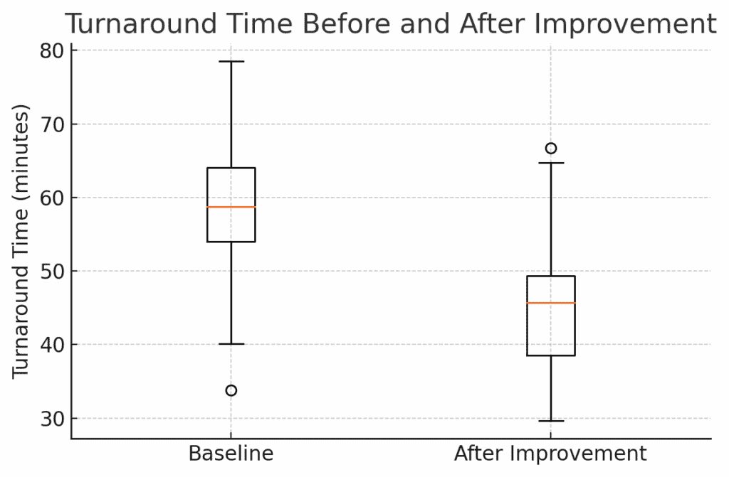
Figure: Turnaround Time Before and After Improvement. This boxplot shows the distribution of room turnover times for a sample of rooms before the changes (left) and after (right). The median dropped from ~58 minutes to ~45 minutes (orange line), and the spread of times narrowed. The improvement is clearly visible (the entire box has shifted down), confirming that the solutions had a strong effect.

In the boxplot above, not only has the average come down, but we also see fewer extreme long delays. This suggests our solutions addressed both typical cases and the occasional worst-case scenarios. Harpreet’s result of ~45 min average is a ~15 min reduction, which in a hospital means a lot. Those 15 minutes per room might translate to a capacity to serve a few more patients daily or reduce backup in the ER. We should quantify this benefit: e.g. if 10 rooms turn over each day, that’s 150 minutes saved per day. That’s like creating an extra 2.5 hours of room availability daily. That could easily be 2 to 3 extra patient admissions per day as Harpreet observed.

  • Document the Changes: As improvements are implemented, update standard operating procedures (SOPs), checklists, or any policy documents. If a new software alert is used, ensure everyone is trained on it. Basically, incorporate the solutions into the normal workflow of the hospital. Harpreet’s checklist should become part of the routine room cleaning protocol for all staff going forward.

Why focus on these points in Improve? Because generating a range of ideas and piloting ensures we find an optimal solution, not just the first solution. It also engages the team. People are more committed to changes they helped design. Validating with data is crucial to prove that the improvement is real and not just a one-time fluke or placebo. As the DMAIC approach emphasizes, you compare the post-improvement data to the baseline to see the actual gains. This is our evidence that the problem is solved.

Risks if not addressed: If we implement changes without piloting, we might introduce new problems. For example, an automated alert system might spam housekeeping if not tuned, or a poorly designed checklist might slow cleaners down initially. Without measuring after, we might not realize that, say, we only improved to Fifty minutes on average, not the goal of 45, leaving some potential gains on the table.

We also risk not capturing the full benefit: maybe the average went down but there’s still a lot of variation that another tweak could fix. If we don’t validate, we can’t confidently celebrate or know to adjust. Moreover, failing to document the new process could mean the improvements aren’t consistently followed (some staff might ignore the checklist if it’s not official). Not thoroughly executing the Improve phase could result in partial improvement, unanticipated side effects, or difficulty sustaining the changes.

Prepare to Communicate Results

Why: Demonstrating improvement to leadership builds support and encourages further Lean work.

Suggestions: Create a simple before/after comparison table:

MetricBeforeAfter
Mean Room Turnaround Time[Insert baseline][Insert updated value]

Include qualitative wins, like fewer communication complaints.

Risk of not making this change: Leadership may not understand the value generated by the project or may not support scaling it further.

Control: Sustain the Improvement

Plan for Sustainment

Why: Lean Six Sigma improvements must be maintained over time to create lasting change.

Suggestions:

  • Assign a process owner responsible for weekly/monthly monitoring
  • Create a visual dashboard for room turnaround times
  • Hold periodic huddles to discuss trends and issues

Risk of not making this change: Improvements may erode as attention shifts. New staff may not follow the new process without training and accountability.

The final phase, Control, is about making the improvements stick and monitoring the process so it doesn’t revert. This is often where projects struggle. A great improvement is made, but six months later the metric slips back. We want to prevent that.

  • Standardization and Training: Ensure that the new process (checklist, communication protocol, etc.) is standardized across all shifts and units. Train all relevant staff (existing and new hires) on the updated procedures. For example, include the room-turnover checklist in the orientation for new housekeeping staff and nurses. Make it easy to follow. Perhaps a laminated copy of the checklist is posted on each unit.
  • Control Plan: Develop a simple control plan document that outlines what needs to be monitored and who is responsible. This might include: the KPI (room turnaround time) with a target (e.g. keep average <50 min), how often it will be measured (daily or weekly average, monthly report), and actions to take if performance starts slipping. It could also tie into existing hospital performance dashboards.
  • Monitoring and Response: Track the turnaround times continually. A charge nurse or quality analyst might pull weekly reports of average turnaround time. If the times start creeping up toward, say, 55 minutes for two weeks in a row, that should trigger an investigation: Did a part of the process break down? Are there staffing shortages? Essentially, we establish triggers and a response plan so that the gains are maintained.

One useful tool here is a control chart or at least a run chart of the turnaround time over time:
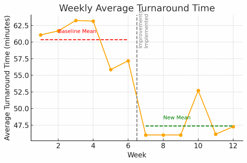
Figure: Weekly Average Turnaround Time after improvements. The orange line shows the average time per week. After Week 6 (when improvements were implemented, marked by the dashed line), the process mean shifts from about 60 min (red line) down to ~47 min (green line). This new level has been maintained for several weeks. A control plan would involve watching this chart going forward. I the line starts trending back up near 60 or beyond acceptable limits, it signals that we need to take corrective action.

In the chart above, we see a stable new performance. Control phase is about keeping it that way. That could involve Statistical Process Control charts, checklists, audits, or other means of verifying the process doesn’t slip. For instance, we might institute a monthly audit where a manager randomly checks 5 cleaned rooms against the checklist to ensure quality hasn’t dropped as speed increased.

  • Assign Process Ownership: Identify a process owner (perhaps the Environmental Services manager or unit manager) who is accountable for this metric. That person ensures the control plan is executed. e.g., they review the data regularly and convene the team if performance declines. They also champion ongoing improvements (maybe the process can be improved further or simplified over time).

Why emphasize Control? Because improvement is not one-and-done. Maintaining gains requires vigilance. Humans naturally fall back into old habits, or new challenges emerge (like staff turnover, or higher patient volumes) that can strain the process.

The control phase makes the new way the default way, through procedures and monitoring. It also provides a safety net. If something starts to go wrong, it will be caught early. Think of it as maintaining a car after you’ve fixed it. You still need oil changes and a dashboard warning light in case of issues.

Risks if not addressed: If we neglect the Control phase, the hospital could quietly slide back to 60-minute turnarounds in a few months. Perhaps a key person leaves and the process knowledge is lost, or people stop using the checklist once the spotlight is off. Without monitoring, it might go unnoticed until patients are waiting again and someone asks “why are we slow again?” By that time, you’ve lost the gains and may have to restart a project.

Also, without control, small problems can snowball. For example, if the alert system fails one day and no one notices, it could introduce delays that become routine. Not having a control plan risks losing all the hard-won improvement, reducing trust in Lean Six Sigma, and missing opportunities to continuously improve further. As the saying goes, “trust but verify.” We trust our improvements, but we must verify over time that they remain effective.

Conclusion

Harpreet’s project is a terrific example of how Lean Six Sigma tools can make a real difference in healthcare operations. We walked through defining the problem in clear terms, measuring it with data, analyzing for root causes, implementing solutions, and then controlling to sustain the win. By applying these steps, we not only achieve the immediate result, but also ensure the hospital can maintain and build on that success. This means consistently faster admissions and more patients served without adding beds.

For students learning Six Sigma, it’s incredibly helpful to see a real-life project like this, end-to-end. It bridges the gap between theory and practice. And even for experienced practitioners, sometimes an outside eye or a structured review can reveal tweaks to get even more value from a project.

What do you think? If you have other suggestions for things Harpreet might try or analyze, please reply in the comments! Perhaps you have insight from a similar project, your input can help everyone learn.

Finally, if you’d like to see another detailed project walk-through in your industry (whether it’s healthcare, manufacturing, finance, etc.), let us know. I’m happy to do another case study breakdown for a student project. Having an example that hits close to home can be a powerful learning tool. Lean Six Sigma is continuous improvement, and we’re all in it together to share and grow.

When you’re ready, there are a few ways I can help:

First, join 12,000+ other Six Sigma professionals by subscribing to my email newsletter. A short read every Monday to start your work week off correctly. Always free.

* * *

If you’re looking to pass your Six Sigma Yellow Belt, Green Belt or Black Belt exam, I’d recommend starting with my affordable study guide:

1)→ 🟡Pass Your Six Sigma Yellow Belt: built for ASQ, IASSC and ILSSI, 1,700+ practice questions with explanations, and six full-length mock exams for your exam

2)→ 🟢Pass Your Six Sigma Green Belt: a study guide organized by the exam Body of Knowledge, 1,300+ practice questions with detailed answer explanations, and 20 full-length mock exams

3)→ ⚫Pass Your Six Sigma Black Belt: the full Black Belt Body of Knowledge, 2,200+ practice questions with detailed answer explanations, and 20 full-length mock exams

You’ve spent so much effort learning Lean Six Sigma. Why leave passing your certification exam up to chance? This comprehensive study guide offers 1,700+ exam-like questions for Yellow Belts, 1,300+ for Green Belts and 2,200+ for Black Belts with full answer walkthroughs, access to instructors, detailed study material, and more.

​ Thousands have used this system to prepare. Join them here. 
Chi-Square Test of Independence

The chi-square test of independence (also called a chi-square test of association) determines whether two categorical variables are statistically independent of each other.

In Six Sigma, this is extremely useful for analyzing contingency tables. For example, you might want to see if defect occurrence is independent of the shift, or if customer satisfaction ratings are independent of location. It helps answer questions like, “Are these two factors related, or are any differences just random variation?”

When to Use a Chi-Square Test of Independence

Use a chi-square test of independence in the Analyze phase when you have counts of outcomes classified by two categorical factors, and you suspect there may be a relationship. For instance, you collected data on defects categorized by machine and defect type. Is the pattern of defect types the same for each machine (independence)? Or does one machine have disproportionately more of certain defects (dependence)? Another example: a call center manager might check if call resolution outcome is independent of the agent’s experience level. Essentially, whenever you have an R×C table of counts (R rows = categories of variable1, C columns = categories of variable2), this test can tell you if there’s an association.

Hypotheses:

  • H₀: The two categorical variables are independent (no association). In other words, the distribution of one variable is the same for all categories of the other variable.
  • H₁: The two variables are not independent (there is an association). At least some categories of one variable are linked to differences in the distribution of the other.

Assumptions: As with the GOF test, the observations should be independent of each other. The sample should also be large enough that expected counts are at least 5 in each cell, or at least in the vast majority of cells. If any cell has an expected count too low, results may not be reliable (you might combine sparse categories or use Fisher’s exact test for a 2×2 table if necessary).

The data for an independence test are typically arranged in a contingency table. Each cell of the table contains the count of observations that fall into the corresponding row category and column category combination. For example, rows might be “Machine A vs Machine B” and columns “Defect Type X, Y, Z,” with each cell showing how many defects of each type occurred on each machine.

Steps to Perform a Chi-Square Test of Independence

  1. Set up hypotheses:
    • Null (H₀): The two variables are independent (no association between them).
    • Alternative (H₁): The two variables are associated (the distribution of one depends on the other).
  2. Choose significance level (α): Often 0.05.
  3. Create the contingency table of observed counts: Organize your data into a table of r rows and c columns. Calculate the row totals, column totals, and the grand total n. These totals are needed to compute expected counts.

Calculate the Statistic and Decide

  1. Calculate expected counts for each cell: If H₀ is true (independence), the expected frequency in a cell is:
    Eij = (Row i total × Column j total) / n
    This comes from probability theory: if events are independent, P(row i and col j) = P(row i)*P(col j), so expected count = (row proportion * column proportion * n). You do this for every cell. For example, suppose 60% of survey responses came from Region A (row) and 30% preferred Product X (column). Under independence you would expect 0.6 * 0.3 = 18% of all respondents to fall in the (Region A, Product X) cell.
  2. Compute the chi-square statistic: Sum over all cells:
    χ² = Σ (Oij − Eij)² / Eij, summed over all r rows and c columns
    Each cell’s contribution is calculated similarly to the GOF test, comparing observed vs expected.
  3. Degrees of freedom: df = (number of rows – 1) × (number of columns – 1). This formula reflects that once you know all the row and column totals, only that many cells are free to vary independently; the rest are determined by totals.
  4. Find the critical value (right-tailed): Use the χ² table for the given df at your α. This test is right-tailed: large χ² means observed counts diverge from expected (indicating dependence). Alternatively, calculate the p-value corresponding to the χ² statistic and df.
  5. Conclusion: If χ²_stat > χ²_critical (p < α), reject H₀. Conclude there is a significant association between the two variables: the differences in the contingency table are unlikely due to chance. If χ²_stat is not beyond critical (p ≥ α), fail to reject H₀, meaning you do not have evidence of an association (the variables could be independent).

Independence Test Example: Process Defects by Shift

As a Six Sigma example, suppose a manufacturing team wants to know if the occurrence of defect types is independent of the production shift (Day shift vs. Night shift). They categorize defects into three types: Type A, Type B, Type C. Over a month, they collect the following data:

  • Day Shift: 16 defects of Type A, 4 of Type B, 10 of Type C (Total = 30 defects in day shift).
  • Night Shift: 8 defects of Type A, 12 of Type B, 10 of Type C (Total = 30 defects in night shift).
    (Total defects observed = 60.)

The contingency table of observed counts would be:

Type AType BType CRow Total
Day Shift1641030
Night Shift8121030
Col Total24162060

We’ll test at 95% confidence (α = 0.05) if shift and defect type are independent.

Solving the Example Step by Step

Step 1. Hypotheses:
H₀: Defect type is independent of shift (no relationship between shift and defect distribution).
H₁: Defect type depends on shift (the pattern of defect types differs between day and night shifts).

Step 2. Significance: α = 0.05.

Step 3. Observed data: (as in the table above).

Step 4. Expected counts: Compute for each cell using E = (row total * col total) / grand total. For example:

  • Day/A: (Day total 30 * Type A total 24) / 60 = 12.
  • Day/B: (30 * 16) / 60 = 8.
  • Day/C: (30 * 20) / 60 = 10.
  • Night/A: (30 * 24) / 60 = 12.
  • Night/B: (30 * 16) / 60 = 8.
  • Night/C: (30 * 20) / 60 = 10.

So the expected table (under H₀) would be:

Type AType BType CRow Total
Day (Exp)1281030
Night (Exp)1281030
Col Total24162060

Chi-Square Statistic and Conclusion

Step 5. Χ² calculation: Sum (O−E)²/E for all 6 cells:

  • Day/A: (16−12)²/12 = (4)²/12 = 16/12 = 1.33
  • Day/B: (4−8)²/8 = (−4)²/8 = 16/8 = 2.00
  • Day/C: (10−10)²/10 = 0
  • Night/A: (8−12)²/12 = (−4)²/12 = 16/12 = 1.33
  • Night/B: (12−8)²/8 = (4)²/8 = 16/8 = 2.00
  • Night/C: (10−10)²/10 = 0

χ²_stat = 1.33 + 2.00 + 0 + 1.33 + 2.00 + 0 = 6.67 (approximately).

Step 6. Degrees of freedom: df = (2-1)*(3-1) = 1 * 2 = 2.

Step 7. Critical value: For df = 2 and α = 0.05 (right-tailed), χ²_critical = 5.991.

Step 8. Conclusion: Our χ²_stat = 6.67 which is greater than 5.991. That means p-value < 0.05. We reject H₀ and conclude there is a significant association between shift and defect type. In practical terms, the mix of defect types is different on day vs. night shift. Looking at the observed vs expected, Day shift had more Type A than expected and fewer Type B, whereas Night shift had more Type B and fewer Type A than expected. This insight suggests that shift (perhaps the conditions or personnel on each shift) has an impact on what kinds of defects occur. That information can guide further root cause analysis (maybe day shift has an issue causing Type A defects, while night shift struggles with Type B).

(Note: If our χ²_stat had been less than 5.991, we’d conclude there’s no evidence of a difference. The defect pattern could be essentially the same on both shifts.)

What the Result Means for the Project

This example shows how the chi-square test of independence finds relationships between categorical factors in a process. In a Six Sigma project, such a finding would prompt an investigation into why the association exists. For example, do day and night shifts follow different procedures, or do they have different skill levels that lead to certain defects? Either way, it is an Analyze phase tool for confirming or ruling out a suspected factor-effect relationship.

(In this test, as with GOF, we used the right tail of the χ² distribution. A large χ² (here ~6.67) beyond the cutoff signaled a significant difference. Independence tests are always right-tailed because only greater divergence (not a deficiency) indicates dependence.)

A Second Example: When the Test Says “No Association”

The example above found a real association (we rejected H₀). It’s just as important to see what it looks like when the test says the opposite: the variables really do look independent. Exam questions test both outcomes, not just the “reject” case.

Suppose a plant wants to know whether meeting spec is independent of which of two production lines made the part. Over a week, they collect:

Meets SpecDoes Not Meet SpecRow Total
Line 17624100
Line 28020100
Col Total15644200

H₀: Meeting spec is independent of production line. H₁: Meeting spec depends on which line made the part. α = 0.05.

Expected counts (row total × column total ÷ grand total): For Line 1, Meets = (100×156)/200 = 78 and Not = (100×44)/200 = 22. Line 2 has the same row total, so its expected counts are also 78 and 22. All four expected counts are comfortably above the minimum of 5 needed for this test to be reliable.

Chi-square statistic: (76−78)²/78 + (24−22)²/22 + (80−78)²/78 + (20−22)²/22 = 0.05 + 0.18 + 0.05 + 0.18 ≈ 0.47.

Degrees of freedom: (2−1)×(2−1) = 1. Critical value at df = 1, α = 0.05: 3.841.

Conclusion: 0.47 is far below 3.841, so we fail to reject H₀. There’s no evidence that meeting spec depends on which line made the part; the small differences between the two lines are consistent with normal random variation. Notice this is a 2×2 table, the most common shape you’ll actually see on an exam question.

Download Chi-Square Test of Independence Excel Exemplar

Unlock Additional Members-only Content!

To unlock additional content, please upgrade now to a full membership.
Upgrade to a Full Membership
If you are a member, you can log in here.

When you’re ready, there are a few ways I can help:

First, join 12,000+ other Six Sigma professionals by subscribing to my email newsletter. A short read every Monday to start your work week off correctly. Always free.

* * *

If you’re looking to pass your Six Sigma Yellow Belt, Green Belt or Black Belt exam, I’d recommend starting with my affordable study guide:

1)→ 🟡Pass Your Six Sigma Yellow Belt: built for ASQ, IASSC and ILSSI, 1,700+ practice questions with explanations, and six full-length mock exams for your exam

2)→ 🟢Pass Your Six Sigma Green Belt: a study guide organized by the exam Body of Knowledge, 1,300+ practice questions with detailed answer explanations, and 20 full-length mock exams

3)→ ⚫Pass Your Six Sigma Black Belt: the full Black Belt Body of Knowledge, 2,200+ practice questions with detailed answer explanations, and 20 full-length mock exams

You’ve spent so much effort learning Lean Six Sigma. Why leave passing your certification exam up to chance? This comprehensive study guide offers 1,700+ exam-like questions for Yellow Belts, 1,300+ for Green Belts and 2,200+ for Black Belts with full answer walkthroughs, access to instructors, detailed study material, and more.

​ Thousands have used this system to prepare. Join them here. 
Sample Size

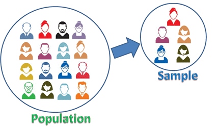
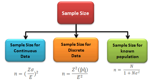
Sample size determination is the mathematical estimation of the number of population units considered for the study. In other words, it tells you how many units to put in the sample, the subset of the population you use to make inferences about the population. The sample must be adequate to represent the population.

Sample Size

How Large Should a Data Sample Be?

The sample size is the number of observations collected from a population; it is a subset of the population to make inferences about the population. Moreover, determining sample size is an important element of every survey based on sampling.

When you pick an SS, there will always be a tradeoff between precision and cost. This trade-off depends on:

Sample size needed for hypothesis testing depends on:

  • Desired Risk (Both alpha and beta)
  • The minimum value to be detected between the population means
  • The population variance is the variation in the measured characteristic (S or sigma).
  • Population size usually does NOT affect how big the sample needs to be. It matters only when the sample is a large share of a finite population, where a finite population correction applies.

Why Use Data Sampling?

Sometimes trying to gather information on a complete population is too expensive, time-consuming, or nonsensical.

For example, we might take samples when:

  • The process we are measuring would require destructive testing (think taste tests, car crash tests, etc.)
  • Getting data from the entire population is too expensive or would take longer than we have.
  • Getting total population data is just too hard.

For example, CNN’s coverage of an election cycle in the United States makes it impossible to ask every voter how they voted. Even if it were, not all would answer. Instead, they use exit polls to derive statistical conclusions about the population as a whole. In a DMAIC sense, this is most common in the Measure phase.

We would unlikely use sampling when the events and products are unique and cannot be replicable.

To get around these constraints, black belts or statisticians extract the samples from the statistical population and make inferences about the population.

Factors Affecting Sample Size(SS)

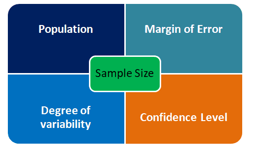
In a quantitative study, SS selection depends on the population, the margin of error, the confidence level, and the degree of variability.

Sample Size

Population: Population is the group of elements which has common characteristics. It is a collection of observations we would like to make inferences about.

Sample: A sample is the subset of the population

Margin of Error

The margin of error is a statistic expressing the amount of random sampling error in the results of an experiment. It determines how much higher or lower the population means you are willing to let your sample mean fall. Often margin error is expressed in terms of percentage.

Confidence Level

The Confidence level is the estimated probability that a population estimate lies within a given margin of error. In other words, it tells how confident you want to be that the actual mean falls within your margin of error of the sample mean. The most commonly used confidence levels are 90%, 95%, and 99%.

Degree of variability

The degree of variability is how spread out the values are in the population, measured by the standard deviation (or by p(1 – p) for a proportion). The greater the variance, the larger the sample size.

How to Calculate a Sample Size

Regarding Six Sigma, we are usually trying to determine an appropriate sample size for doing one of two things; estimate an average or a proportion. The equation you use to determine your SS depends on what you’re going to do with that sample.

Either way, the variables are as follows:

n = sample size (what we’re solving for)

d (Sometimes represented as delta or Δ) = precision = the range for an estimate of a characteristic = half the width of a confidence interval.

Precision in this sense can be a bit tricky, so here are a few examples;

  • Estimate of a lead time of +/- 4 days
    • precision would = 4 days.
  • Estimate of a percent rejected +/- 10%
    • precision would = 10%
  • 95% CI (4,10) for a lead time in hours.
    • Estimate of a lead time between 4 and 10 hours
    • Width of the confidence interval would be = 10-4 hours = 6 hours
    • precision = d = 1/2 of C.I. width = 6/2 = 3 hours

Sample Size(SS) calculation decision guide

  • Sample size determination is the mathematical estimation of the number of population units to be included in the study. It must be adequate to represent the population. The determination should be optimum and has to be obtained by the scientific method.
  • If the SS is 30 or more, it is known as a large sample
  • For large samples, the sampling distribution of the mean is approximately normal (central limit theorem), so we use the Z distribution
  • For small samples (<30) with an unknown σ, use the t distribution for a mean. The F and chi-square distributions are used for variances at any sample size.
  • The value of statistics obtained from a large sample can be taken as an estimation of the population parameters.
Sample Size

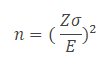
Sample Size for One Sample, Continuous Outcome

Where n is the SS, Z is the Z score from the desired risk, sigma is the standard deviation, and E is the mean shift, or error.

Example: A Peanut Butter Manufacturer wants to estimate the sugar content in a bottle. In fact, the previous batch of 1000 bottles had a standard deviation of 10 gms. Identify the sample size to estimate the mean is within 4 gms of the population mean with a 95% confidence.

  • Margin of error E = 4gm
  • Standard deviation = 10gm

First, we need to identify the alpha

Subtract the confidence level (95%) from 1 to get alpha, then divide alpha by two to get α/2

α = 1 – 0.95 = 0.05, so α/2 = 0.05/2 = 0.025

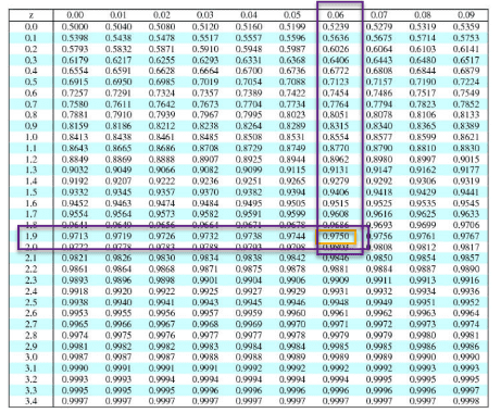
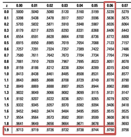
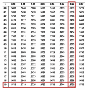
This page uses a cumulative z table: each value is the area to the left of z, which is why the next step looks up 0.975 to get 1.96. If your handbook’s table shows the area from the mean (0 to z), look up 0.475 instead; if it shows the upper tail, look up 0.025.

Next, subtract α/2 from 1 and look that value up in the body of the z table to get the z-score

1-0.025 =0.975

Z-score=1.96

So, Sample size n =  (z* σ/E)2 = (1.96* 10/4)2 = 24.01, which rounds up to 25. Always round a sample size up to the next whole number, or the sample will fall slightly short of the precision you asked for.

Also see: https://sphweb.bumc.bu.edu/otlt/mph-modules/bs/bs704_power/BS704_Power3.html

Sample Size for Continuous and Binary Random Variables

Where

n = SS

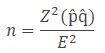
p̂ is the estimated proportion. If you have no estimate, use 0.5, which gives the largest sample size.

q̂=1- p̂

Example: The expectation is that 20% of employees in the New York area are using Subway. With 90% confidence level, what would be the minimum sample that needs to estimate the population proportion with a maximum permissible difference of 6%?

Sample proportion=0.20

Margin of error E =0.06

90% confidence level α = 1-0.90 = 0.1; Z =1.645

So, SS = p̂ (1- p̂)* (Z/E)2 = 0.2*(1-0.2)* (1.645/0.06)2 = 120.26 =121.

Also, see:

(Cochran’s formula) https://www.statisticshowto.com/probability-and-statistics/find-sample-size/

Sample Size for Known populations (Slovin’s Formula)

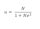
Slovin’s formula is used to compute the sample size in a study for a given total population and a margin of error. Slovin’s formula works for simple random sampling. It assumes a known population size, a proportion near 0.5 and about 95% confidence. If those do not hold, use the formula above (Cochran’s formula) with a finite population correction.

Where

n = sample size

N= total population

e=margin of error

Example: Compute the SS for a population of 1200. You need to take a survey about financial problems. While the margin of error is 5%.

Population N =1200

Margin of error E =0.05

So, SS = N/(1+Ne2)= 1200/(1+1200*0.052) =1200/4=300.

https://opentextbc.ca/introbusinessstatopenstax/chapter/calculating-the-sample-size-n-continuous-and-binary-random-variables

SS for Discrete Data

Also see: SS for a Known or Finite Population

https://blog.remesh.ai/how-to-calculate-sample-size

https://www.calculator.net/sample-size-calculator.html

How to Find a SS Given a Confidence Level and Width (known population standard deviation): https://www.statisticshowto.com/probability-and-statistics/find-sample-size/

Also see: SS for an Unknown or Infinite Population

https://www.surveymonkey.com/mp/sample-size-calculator/

Also see: SS for Other Data Types (Nominal, Ordinal, Interval, Ratio)

See:

How to Calculate SS Videos

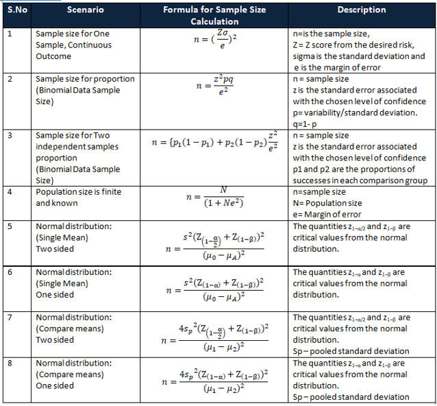
Formulas for various scenarios

Sample Size and Hypothesis Tests, Designed Experiments

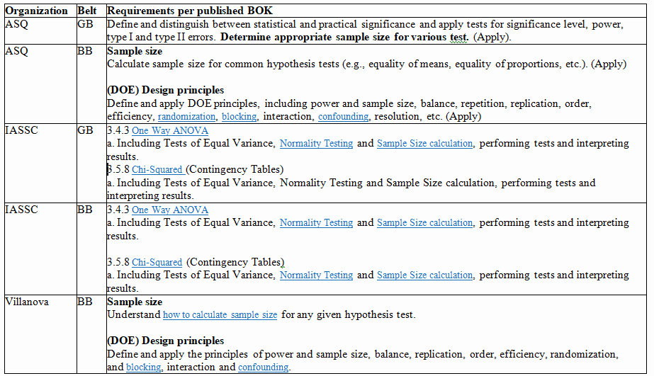
In addition to basic SS calculations, Six Sigma candidates are often required to understand how to calculate appropriate SS for use in hypothesis tests and in Designed Experiments. Here are 2 charts I’ve assembled taken from requirements explicitly stated in the ASQ, IASSC, & Villanova Green Belt and Black Belt BOKs.

When you’re ready, there are a few ways I can help:

First, join 12,000+ other Six Sigma professionals by subscribing to my email newsletter. A short read every Monday to start your work week off correctly. Always free.

* * *

If you’re looking to pass your Six Sigma Yellow Belt, Green Belt or Black Belt exam, I’d recommend starting with my affordable study guide:

1)→ 🟡Pass Your Six Sigma Yellow Belt: built for ASQ, IASSC and ILSSI, 1,700+ practice questions with explanations, and six full-length mock exams for your exam

2)→ 🟢Pass Your Six Sigma Green Belt: a study guide organized by the exam Body of Knowledge, 1,300+ practice questions with detailed answer explanations, and 20 full-length mock exams

3)→ ⚫Pass Your Six Sigma Black Belt: the full Black Belt Body of Knowledge, 2,200+ practice questions with detailed answer explanations, and 20 full-length mock exams

You’ve spent so much effort learning Lean Six Sigma. Why leave passing your certification exam up to chance? This comprehensive study guide offers 1,700+ exam-like questions for Yellow Belts, 1,300+ for Green Belts and 2,200+ for Black Belts with full answer walkthroughs, access to instructors, detailed study material, and more.

​ Thousands have used this system to prepare. Join them here. 
Two Sample Z Test of Proportions

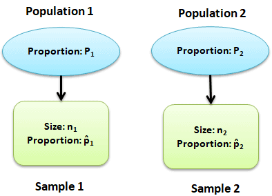
Two sample Z test of proportions is the test to determine whether the two populations differ significantly on specific characteristics. In other words, compare the proportion of two different populations that have some single characteristic. It checks whether the gap between the two sample proportions is too large to be chance. A confidence interval for p1 – p2 gives the range of likely values for that gap.

Two Sample Z Test of Proportions

For example, compare the proportion of men baseball players who are right-handed to the proportion of women baseball players who are right-handed.

When to use Two Sample Z Proportion test

The purpose of two sample Z test is to compare the random samples of two populations. Use two sample z test of proportion for large sample size and Fisher exact probability test is an excellent non-parametric test for small sample sizes.

Assumptions of the Two Sample Z Proportion Hypothesis Tests

  • The data are simple random values from both the populations
  • Both populations follow a binomial distribution
  • Samples are independent of each other
  • Test results are accurate when np and n(1-p) are greater than 5

Hypothesis of two sample Z proportion test

  • Null hypothesis: The difference between population proportions is equal to hypothesized difference
  • Alternative hypothesis: The difference between population proportions is not equal to hypothesized difference (two -tailed)
  • The difference between population proportions is greater than hypothesized difference (right-tailed)
  • The difference between population proportions is less than hypothesized difference (left -tailed)

Two Sample Z Test of Proportions Variations

There are 2 ways to compute the two sample Z test of proportions i.e pooled or unpooled. Use the pooled formula only when H0 says p1 = p2. For a nonzero hypothesized difference, use the unpooled standard error. Some courses, such as IASSC, use the unpooled form for p1 = p2 too.

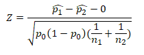
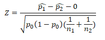
Pooled Z test of proportions formula

Pooled Calculation

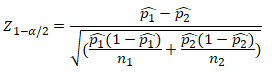
Un-pooled Z test of proportions formula

Two Sample Z Test of Proportions
Unpooled Calculation

Procedure to execute Two Sample Proportion Hypothesis Test

  • State the null hypothesis and alternative hypothesis
  • State alpha, in other words determine the significance level
  • Compute the test statistic
  • Determine the critical value (from critical value table)
  • Define the rejection criteria
  • Finally, interpret the result. If the test statistic falls in critical region, reject the null hypothesis

Two Sample Z Test of Proportions Pooled (ASQ, Villanova)

Two Sample Z Test of Proportions

Where

The one and two sample proportion hypothesis
  • z is test statistic
  • p̂1 and p̂2 are observed proportion of events in the two samples
  • n1 and n2 are sample sizes
  • X1 and X2 are the number of events (successes) in each sample

Example of Two Sample Z Proportion Test (pooled)

Example: A car manufacturer aims to improve the quality of the products by reducing the defects and also increase the customer satisfaction. Therefore, he monitors the efficiency of two assembly lines in the shop floor. In line A there are 18 defects reported out of 200 samples. While the line B shows 25 defects out of 600 cars. At α 5%, is the differences between two assembly procedures are significant?

Define Null and Alternative hypothesis

  • Null Hypothesis: Two proportions are the same
  • Alternative Hypothesis: Two proportions are not the same

α=0.05

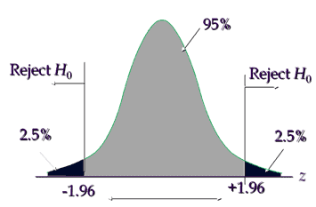
State decision rule

Example of  Two Sample Proportion  Test
Two Sample Z Test of Proportions

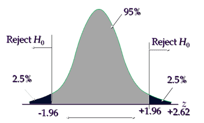
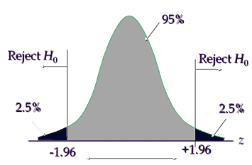
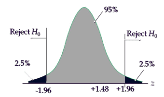
Critical value is ±1.96, hence reject the null hypothesis if the calculated value is less than -1.96 or greater than +1.96

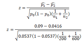
Calculate Test Statistic

  • Line A= p̂1=18/200= 0.09 = 9%
  • Line B= p̂2 = 25/600 = 0.0417 = 4.17%
  • First compute p0 = (18+25)/(200+600) = 43/800 = 0.0537 =5.37%
  • Now p̂1 – p̂2 = 0.09 – 0.0416 = 0.0484
  • p0 * (1 – p0 ) = 0.0537 * (1-0.0537) = 0.0537 * 0.9463 = 0.0508
  • And (1/n1) + (1/n2) = 0.006667
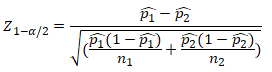
  • So, Z = (0.0484)/ SQRT ( (0.0508) * (0.006667))
  • Z = (0.0484)/ SQRT ( 0.000339)) = (0.0484)/ (0.018406) = 2.62
Two Sample Z Test of Proportions

Interpret the results: Compare Zcalc to Zcritical . In hypothesis testing, a critical value is a point on the test distribution compares to the test statistic to determine whether to reject the null hypothesis. Calculated test statistic value 2.62 and it is in critical region, hence reject the null hypothesis, so, there is a significant difference in two line assembly procedures.

Pooled Z test of proportions formula template

Unlock Additional Members-only Content!

To unlock additional content, please upgrade now to a full membership.
Upgrade to a Full Membership
If you are a member, you can log in here.

Two Sample Z Test of Proportions Pooled (ASQ, Villanova) Helpful Videos

https://www.youtube.com/watch?v=_58qBy9Uxks

Two Sample Z Test of Proportions Un-Pooled (IASSC)

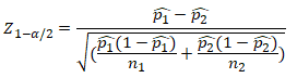
  • z is test statistic
  • p̂1 and p̂2 are observed proportion of events in the two samples
  • n1 and n2 are sample sizes

Example of Two Sample Z Proportion Test (Unpooled)

Example: Researchers want to test the side effects of a new COVID vaccine. In clinical trail 62 out of 300 individuals taking X1 vaccine report side effects. While 48 individuals out of 300 taking X2 vaccine report side effects. At 95% confidence level, is the X1 vaccine working any differently than the X2?

Define Null and Alternative hypothesis

  • Null Hypothesis: Two proportions are the same
  • Alternative Hypothesis: Two proportions are not the same

α=0.05

State decision rule

Critical value is ±1.96, hence reject the null hypothesis if the calculated value is less than -1.96 or greater than +1.96

Calculate Test Statistic

  • Vaccine X1= p̂1 = 62/300 = 0.2067
  • Vaccine X2 =p̂2= 48/300 = 0.16
  • n1 and n2=300
  • Now p̂1 – p̂2 = 0.2067 – 0.16 = 0.0467
  • p̂1 (1- p̂1)/n1 = (0.2067*(1-0.2067)) /300 = 0.000547
  • And p̂2 (1- p̂2)/n2 = (0.16*(1-0.16)) /300 = 0.000448
  • Sqrt( (p̂1 (1- p̂1)/n1)+ (p̂2 (1- p̂2)/n2)))= 0.0315
  •  So Z = 0.0467/0.0315 = 1.48

Interpret the results: Compare Zcalc to Zcritical . In hypothesis testing, a critical value is a point on the test distribution compares to the test statistic to determine whether to reject the null hypothesis. Calculated test statistic value 1.48 and it is not in critical region, hence we failed to reject the null hypothesis. There is not enough evidence that the two vaccines differ in their side effect rate.

Unpooled Z test of proportions formula template

Unlock Additional Members-only Content!

To unlock additional content, please upgrade now to a full membership.
Upgrade to a Full Membership
If you are a member, you can log in here.

Six Sigma Black Belt Certification Two Sample Proportion Z Test Questions:

Question: What could be the null hypothesis for a two sample proportion test, if the alternative hypothesis is p1 <p2?

(A) Null hypothesis : p1 > p2
(B) Null hypothesis : p1 = p2
(C) Null hypothesis : p1 < p2
(D) Null hypothesis : p1 ≠ p2

Answer:

Unlock Additional Members-only Content!

To unlock additional content, please upgrade now to a full membership.
Upgrade to a Full Membership
If you are a member, you can log in here.

When you’re ready, there are a few ways I can help:

First, join 12,000+ other Six Sigma professionals by subscribing to my email newsletter. A short read every Monday to start your work week off correctly. Always free.

* * *

If you’re looking to pass your Six Sigma Yellow Belt, Green Belt or Black Belt exam, I’d recommend starting with my affordable study guide:

1)→ 🟡Pass Your Six Sigma Yellow Belt: built for ASQ, IASSC and ILSSI, 1,700+ practice questions with explanations, and six full-length mock exams for your exam

2)→ 🟢Pass Your Six Sigma Green Belt: a study guide organized by the exam Body of Knowledge, 1,300+ practice questions with detailed answer explanations, and 20 full-length mock exams

3)→ ⚫Pass Your Six Sigma Black Belt: the full Black Belt Body of Knowledge, 2,200+ practice questions with detailed answer explanations, and 20 full-length mock exams

You’ve spent so much effort learning Lean Six Sigma. Why leave passing your certification exam up to chance? This comprehensive study guide offers 1,700+ exam-like questions for Yellow Belts, 1,300+ for Green Belts and 2,200+ for Black Belts with full answer walkthroughs, access to instructors, detailed study material, and more.

​ Thousands have used this system to prepare. Join them here. 
What is the Coefficient of Contingency?

The Coefficient of Contingency (C) measures the strength of association between two categorical variables using data arranged in a contingency table.

It is derived from the Chi-Square test statistic, which tests whether two categorical variables are independent.

In simple terms:

  • Chi-Square tells you if a relationship exists
  • Coefficient of Contingency tells you how strong the relationship is

This makes it an effect size measure for categorical data.

When It Is Used

The coefficient is useful when analyzing relationships between variables such as:

Variable 1Variable 2
MachineDefect Type
ShiftError Rate Category
SupplierQuality Grade
DepartmentTraining Level

These are non-numeric categories, which means traditional correlation methods do not apply.

Understanding Contingency Tables

The coefficient is calculated from a contingency table, which summarizes the frequency distribution of two categorical variables.

Example Contingency Table

Imagine a manufacturing team studying whether machine type affects defect occurrence.

MachineDefectNo DefectTotal
Machine A2080100
Machine B4060100
Total60140200

This table allows us to analyze whether defects occur independently of machine type.

In Six Sigma, this type of analysis commonly occurs during the Analyze phase of
DMAIC.

The Coefficient of Contingency Formula

The coefficient is calculated from the Chi-Square statistic.

The formula is:

[
C = \sqrt{\frac{\chi^2}{\chi^2 + n}}
]

Where:

  • C = Coefficient of Contingency
  • χ² = Chi-Square statistic
  • n = total sample size

This equation scales the Chi-Square value into a range between 0 and less than 1.

Visual Formula Breakdown

ComponentMeaning
χ²Measures deviation from independence
nNumber of observations
RatioAdjusts Chi-Square for sample size
Square rootNormalizes the scale

Why the Coefficient Never Reaches 1

One of the most confusing aspects of this metric is that it never equals 1, even when variables are perfectly associated.

This happens because the maximum value depends on the size of the contingency table.

The theoretical maximum is:

[
C_{max} = \sqrt{\frac{k-1}{k}}
]

Where k is the smaller dimension of the contingency table.

Example

For a 2×2 table:

[
C_{max} = \sqrt{\frac{1}{2}} = 0.707
]

Meaning the largest possible value is only 0.707, not 1.

Because of this limitation, many statisticians prefer Cramer’s V when comparing different table sizes.

Step-by-Step Calculation Example

Let’s calculate the coefficient using the earlier defect example.

Step 1: Observed Data

MachineDefectNo DefectTotal
A2080100
B4060100
Total60140200

Step 2: Calculate Expected Frequencies

Expected frequency formula:

[
E = \frac{(Row\ Total)(Column\ Total)}{n}
]

Example:

For Machine A / Defect:

[
E = \frac{100 \times 60}{200} = 30
]

Expected table:

MachineDefectNo Defect
A3070
B3070

Step 3: Calculate Chi-Square

[
\chi^2 = \sum \frac{(O – E)^2}{E}
]

CellOECalculation
A Defect20303.33
A No Defect80701.43
B Defect40303.33
B No Defect60701.43

Total:

[
\chi^2 = 9.52
]


Step 4: Calculate Coefficient of Contingency

[
C = \sqrt{\frac{9.52}{9.52 + 200}}
]

[
C = \sqrt{0.045}
]

[
C \approx 0.21
]

Interpreting the Coefficient

Unlike correlation coefficients, there are no universal interpretation thresholds.

However, practitioners often use approximate ranges:

CoefficientInterpretation
0.00-0.10Very weak association
0.10-0.30Weak association
0.30-0.50Moderate association
0.50+Strong association

In the example:

C = 0.21

This suggests a weak association between machine type and defects.

This means:

  • Machine type may contribute to defects
  • But it is likely not the primary root cause

Role in Six Sigma Analysis

The coefficient of contingency is particularly useful in the Analyze phase of Six Sigma projects.

It helps teams quantify relationships between categorical variables.

Typical Applications

Defect Root Cause Analysis

VariableExample
MachineDefect type
OperatorError category
SupplierPart failure

Customer Experience Analysis

VariableExample
RegionComplaint type
Product versionReturn reason

Process Investigation

VariableExample
ShiftQuality outcome
Training statusError frequency

These analyses support the goal of identifying statistically meaningful relationships before implementing improvements.

DMAIC Case Study Example

Problem

A call center noticed higher customer complaints on certain shifts.

The Six Sigma team wanted to determine whether shift assignment influences complaint type.

Data Collected

ShiftBilling ComplaintService ComplaintOther
Morning403020
Afternoon203525
Night102030

Total observations = 210

Step 1: Conduct Chi-Square Test

The test shows p < 0.05, indicating complaints vary by shift.

Step 2: Calculate Coefficient of Contingency

The coefficient equals 0.31.

Interpretation

This indicates a moderate association between shift and complaint type.

Root Cause Insight

Further investigation revealed:

  • Night shift agents handled more complex service issues
  • Billing specialists primarily worked morning shifts

The analysis helped the team redesign call routing procedures.

Coefficient of Contingency vs Other Association Measures

Several statistics measure categorical association.

Understanding the differences helps practitioners choose the correct metric.

Comparison Table

StatisticBest ForKey Advantage
Coefficient of ContingencySmall contingency tablesSimple to calculate
Cramer’s VAny table sizeStandardized to 1
Phi Coefficient2×2 tablesEquivalent to correlation
Chi-SquareHypothesis testingDetects existence of relationship

When to Use Cramer’s V Instead

Coefficient of Contingency has a major limitation:

Its maximum value changes with table size.

Cramer’s V solves this problem by standardizing the range from 0 to 1 regardless of dimensions.

For that reason, many modern statistical tools default to Cramer’s V.

However, the coefficient still appears frequently in statistical textbooks and exam questions.

Relationship to Effect Size

In Six Sigma and statistics, effect size measures how meaningful a relationship is.

A statistically significant result does not always mean the effect is important.

Example:

A huge sample size may produce p < 0.001, but the relationship could still be extremely weak.

Coefficient of Contingency helps answer:

“How strong is the relationship?”

This distinction is critical for data-driven decision making.

Practical Tips for Six Sigma Practitioners

Tip 1: Always Pair with Chi-Square

Coefficient of Contingency should never be used alone.

First test for independence using Chi-Square.

Then measure association strength.

Tip 2: Watch Sample Size

Large samples can inflate Chi-Square values.

This may produce misleadingly high coefficients.

Tip 3: Use Visualization

Heatmaps and mosaic plots often reveal patterns faster than raw statistics.

Example visualizations:

  • Contingency heatmaps
  • Mosaic charts
  • Segmented bar charts

Tip 4: Compare with Other Metrics

For deeper analysis, compare results with:

  • Cramer’s V
  • Odds ratios
  • Risk ratios

Each provides a different perspective on the relationship.

Common Pitfalls

Misinterpreting the Range

Because the coefficient cannot reach 1, comparing values across tables can be misleading.

Using with Continuous Data

The coefficient is only for categorical variables.

Continuous data requires different metrics such as:

  • Correlation
  • Regression

Ignoring Expected Frequencies

Chi-Square assumptions require:

  • Expected frequencies ≥ 5 in most cells

Violations may invalidate the analysis.

How This Appears on Six Sigma Certification Exams

Questions typically test:

  • Understanding the formula
  • Interpreting association strength
  • Identifying appropriate use cases

Example exam question:

A contingency table analysis produces:

χ² = 15.3
n = 250

What is the coefficient of contingency?

Using the formula:

[
C = \sqrt{\frac{15.3}{265.3}}
]

[
C \approx 0.24
]

Interpretation:

Weak to moderate association.

This type of question often appears on the Green Belt exam preparation materials such as
https://sixsigmastudyguide.com/pass-your-six-sigma-green-belt/

Key Takeaways

The Coefficient of Contingency is a useful measure for evaluating the strength of association between categorical variables.

Important points to remember:

  • It is derived from the Chi-Square statistic
  • Values range from 0 to less than 1
  • Maximum value depends on table size
  • It measures association, not correlation
  • Best used alongside Chi-Square hypothesis testing

For Six Sigma practitioners, this metric helps quantify relationships uncovered during the Analyze phase, allowing teams to prioritize root causes based on data rather than assumptions.

When you’re ready, there are a few ways I can help:

First, join 12,000+ other Six Sigma professionals by subscribing to my email newsletter. A short read every Monday to start your work week off correctly. Always free.

* * *

If you’re looking to pass your Six Sigma Yellow Belt, Green Belt or Black Belt exam, I’d recommend starting with my affordable study guide:

1)→ 🟡Pass Your Six Sigma Yellow Belt: built for ASQ, IASSC and ILSSI, 1,700+ practice questions with explanations, and six full-length mock exams for your exam

2)→ 🟢Pass Your Six Sigma Green Belt: a study guide organized by the exam Body of Knowledge, 1,300+ practice questions with detailed answer explanations, and 20 full-length mock exams

3)→ ⚫Pass Your Six Sigma Black Belt: the full Black Belt Body of Knowledge, 2,200+ practice questions with detailed answer explanations, and 20 full-length mock exams

You’ve spent so much effort learning Lean Six Sigma. Why leave passing your certification exam up to chance? This comprehensive study guide offers 1,700+ exam-like questions for Yellow Belts, 1,300+ for Green Belts and 2,200+ for Black Belts with full answer walkthroughs, access to instructors, detailed study material, and more.

​ Thousands have used this system to prepare. Join them here.