
What is Six Sigma?

Six Sigma is a framework designed to make an organization more competitive by focusing on being effective and efficient. It is a systematic problem-solving approach centered around defect elimination and variation reduction, leading to process improvement.
What is Six Sigma?

Specifically, Six Sigma is a continuous improvement process with a focus on the following:

  • Change empowerment
  • Smooth training of resources
  • Consistent top management support

Six Sigma refers to the practice of delivering products and services that perform at high standards. It is a Quality Philosophy and a management technique. It is not a standard or a certification. It is also a metric: the sigma level of a process.

Six Sigma’s Basic Premises

The purpose of Six Sigma is to satisfy customers by producing quality products. Hence, it focuses on variation reduction and waste elimination. This leads to increased efficiency.

Variation is the spread of data around the mean. In other words, it is how much process performance varies.

A defect is a measurable product characteristic that does not meet a customer requirement (i.e. defective products). In other words, any process performance outside of the defined specification is a defect. Waste is any activity that adds no value. Defects are one type of waste.

Six Sigma methodologies are used to identify and remove the root cause of defects or reduce the process variation (using statistical or process analysis methods) and also the costs that are associated with it.

For example, let’s say XYZ factory produces widgets. The widgets are all supposed to be a certain size, shape, and weight. Now, randomly sampled output discovers that out of every 1,000 widgets, fifty are flawed (e.g. wrong size, shape, or weight). To correct this, the factory uses Six Sigma to determine what’s causing the variation/defects and works to reduce them to a six-sigma level.

Six Sigma’s Approach to Problem Solving

The term Six Sigma was first coined by American engineer Bill Smith, who is known as the father of Six Sigma. While working at Motorola in the year 1986, Smith created Six Sigma as a general approach to measuring quality in business performance terms. Later, it became a popular management approach at GE with Jack Welch in the early 1990s.
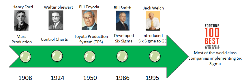
General Electric recognized benefits of $2.5 billion per year due to Six Sigma policies and made it a company-wide strategy. Now, it has become a project-driven approach for process improvements that follows the five-step process, also called the DMAIC cycle. (Also see: History of Continuous Improvement).

Overview Video

What is a Six Sigma Level?

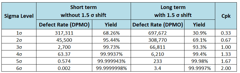
Six Sigma derives from the normal or bell curve in statistics, where each interval indicates one sigma or one standard deviation. Moreover, sigma is a statistical term that refers to the standard deviation of a process around its mean. In a normally distributed process, 99.73% of measurement will fall within ±3σ, and 99.99932% will fall within ±4.5σ.

For a process, the sigma capability is a metric that shows how well that process is performing. Hence the higher the sigma value, the better the process.
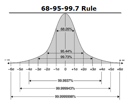
The 68-95-99.7 rule, also known as an empirical rule, is used to remember the percentage of values that lie within a band around the mean in a normal distribution with a width of one, two, and three standard deviations.
What is Six Sigma?

A six sigma capable process will have Cp >= 2.0. Allowing the conventional 1.5 sigma long-term shift of the mean, Cpk >= 1.5 and DPMO = 3.4

Where Does the 6 and Sigma come from?

Let’s cover Sigma first. Sigma, denoted by the symbol σ (a Greek letter), represents the standard deviation of a population. Primarily, it represents the dispersion (or ‘spread’) of a set of data values with respect to mean. A standard deviation is a value you have to calculate and is dependent on the data your process generates.
What is Six Sigma?

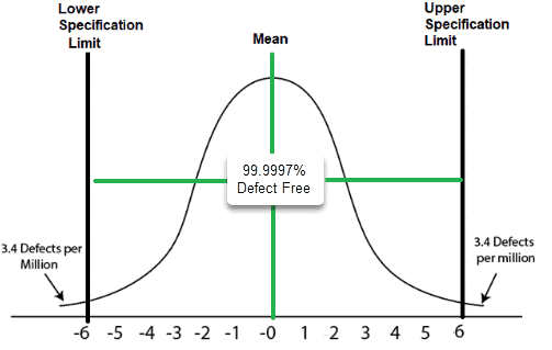
Now let’s cover the 6. The six refers to how many standard deviations away from the mean we set the specification limits in a 6 sigma process.

Now let’s put them together for 6 Sigma: A Six Sigma process has a specification limit that is 6 times its sigma (standard deviation) away from its mean. That is 6 sigma on each side of the mean, so 12 standard deviations fit between the two limits (Cp = 2.0). It is not 3 sigma on each side; that would be a 3 sigma process. Allowing the usual 1.5 sigma long-term shift of the mean, the nearer limit ends up 4.5 sigma away. That is why only about 3.4 defects per million opportunities fall outside the limits we’ve set at 6 sigmas away from the center.

Additionally, you can also think of it as a level of excellence that can be quantified and easily compared against other processes. If you only get 3.4 defects per million opportunities out of your process, i.e. a 99.99966% success rate per opportunity, you have a 6 sigma process.

Other Sigma Levels

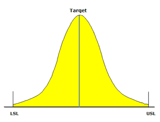
For each standard deviation away from the mean (0 in the graphic above), your process gets more and more defect-free. Let’s look at a 3 Sigma process, for example. In a normally distributed process, if the mean ±3σ range of output is between USL and LSL, then around 99.73% of the points of the output will be non-defective. This is the centered, short-term figure. With the 1.5 sigma shift used for 3.4 DPMO, a 3 sigma process yields about 93.3%.

Is Six Sigma ONLY for Reducing Defects?

Absolutely no! While Six Sigma is primarily known for its focus on reducing defects, it is actually a comprehensive approach to quality improvement that can be applied to a wide range of business processes. In addition to reducing defects, Six Sigma can also be used to improve process efficiency, reduce waste, improve customer satisfaction, and increase profitability.

The core philosophy of Six Sigma is to focus on meeting or exceeding customer expectations by reducing variation and improving process performance. By using statistical tools and data analysis, Six Sigma practitioners can identify the root causes of problems and develop solutions to improve process performance and meet customer needs.

While reducing defects is certainly an important goal in many industries, the broader focus of Six Sigma is to improve overall business performance by reducing variation and improving quality. By improving processes and reducing waste, organizations can increase efficiency, reduce costs, and ultimately deliver greater value to their customers.

The Primary Goals are to Improve

Six Sigma is a data-driven methodology that uses statistical tools and techniques to define the problem and evaluate each process step. In addition, it provides ways to create an efficient business structure, improve the quality of the operations in an organization, and increase the bottom-line profit.

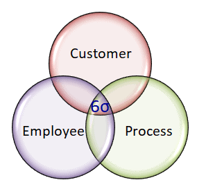
Three Key Elements of Six Sigma

  • Customers: Customers are the key to business, and they are the top priority. Customers define the quality requirements and expect on-time delivery, high performance, great service, and many more. However, meeting customer requirements is not enough in the business world.
  • Process: Defining the process and important metrics is the key aspect of Six Sigma. Since the customer is key for any business, quality needs to be looked at from the customer’s perspective. This helps to identify the gaps in processes and the work necessary to improve them.
  • Employee: Without leadership commitment, using Six Sigma in any organization is difficult. The organization must involve all employees with well-defined roles and clear objectives. Furthermore, organizations must provide required resources like people, training, budget, and more.
What is Six Sigma

Philosophy & Methodology

Six Sigma is a result-oriented, continuous improvement process that includes active involvement from senior management.

Continuous improvement activities in an organization help ensure that problems are identified and solved when they occur. Most of the modern quality improvement models, such as sampling techniques, control charts, process capability, and DOE have been influenced by the theory of continuous improvement.

Why Use Six Sigma?

Organizations face new challenges every day, like rising costs, customer issues, an increase in defect rate, etc. In fact, global competition has made it critical to provide perfect quality at a low cost to keep customers happy and to make organizations viable in the marketplace. Some of the key benefits of using Six Sigma include the following:

  • Creates reliable products and services
  • Ensures customer satisfaction
  • Reduces process variation and eliminates waste
  • Eliminates the root causes of problems and defects in a process
  • Reduces rework by getting it right the first time
  • Addresses key organization business requirements
  • Competitive advantage

Six Sigma Methodologies

Six Sigma provides better value to customers, employees, and all the stakeholders in an organization. Additionally, it is a business initiative that improves quality and productivity and reduces costs.

DMAIC

One of the basic tools in Six Sigma is the use of the DMAIC methodology. (Also see DMAIC Overview). Particularly, DMAIC is a logical framework that helps you think through a process, plan improvements, and achieve a Six Sigma level of quality. In other words, it is a data-driven quality strategy for a better process.

There are five phases in the DMAIC method. They are as follows:
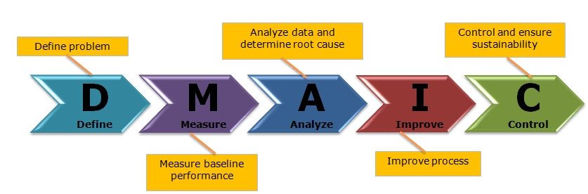
  • Define: Define the problem and also project goals that need to be addressed.
  • Measure: Measure the baseline performance and confirm the practical problem by collecting data
  • Analyze: Analyze the data to determine the root causes of the problems and then identify opportunities for improvements.
  • Improve: Improve the process and test the statistical solution.
  • Control: Start using a new process for production. Implement, control, and ensure sustainability. Finally, measure the new process based on customer reactions.

Six Sigma teams define the problem, work with sponsors and stakeholders, and deliver results that will be reviewed at phase-gate meetings called DMAIC Tollgate Reviews.

DMADV

DMADV is one aspect of Design for Six Sigma (DFSS). In fact, this evolved from the continuous quality improvement and Six Sigma approach to reduce variation. However, DMADV aims to create new processes and new products or services.
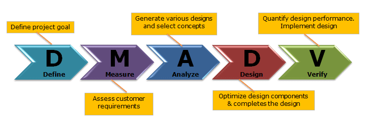
  • Define: Determine the project need and also identify the goals
  • Measure: Assess customer needs and prioritize requirements
  • Analyze: Analyze data, generate various designs, and select concepts
  • Design: Optimize design components and completes the design
  • Verify: Validate and quantify the design performance.

Six Sigma Frequently Asked Questions

What is the concept of Six Sigma?

Six Sigma refers to the methodology and practice of focusing on developing and delivering products/services that perform at high standards. It is a Quality Philosophy and a management technique. It is a systematic problem-solving approach centered around defect elimination and variation reduction, leading to process improvement.

What are the Five steps of six sigma?

  • Define: Define the problem and also project goals that need to be addressed
  • Measure: Measure the baseline performance and validate the practical problem by collecting data
  • Analyze: Analyze the data to determine the root causes of the problems and opportunities for improvement
  • Improve: Improve the process and test the statistical solution
  • Control: Start using a new process for production. Implement, control, and ensure sustainability. Finally, measure the new process based on customer reactions.

Why is it called six sigma?

Sigma, denoted by the symbol σ (a Greek letter), represents the standard deviation of a population. Particularly, it characterizes the dispersion (or ‘spread’) of a set of data values with respect to mean.

A Six Sigma process has a specification limit that is 6 times its sigma (standard deviation) away from its mean. In other words, there are 6 standard deviations between the mean and each specification limit, 12 in all (Cp = 2.0). Allowing the usual 1.5 sigma long-term shift of the mean, the nearer limit is 4.5 sigma away, so only about 3.4 defects per million opportunities fall outside the specification limits that we’ve set at 6 sigmas away from the center.

What is an example of Six Sigma?

Six Sigma means being defect-free in 99.99966% of opportunities, allowing only 3.4 defects per million opportunities.

Also, refer to a few examples of Six sigma implementation:

What are 6 Sigma tools?

  • DMAIC: DMAIC is Six Sigma’s signature framework for process improvement. It provides a structured way of improving a process.
  • 5S: 5S Workplace Organization is a visual system. It is often put in place through a Kaizen event. 5S derives its name from five Japanese terms beginning with the “s” to create a workplace suited for visual control and lean production. 
  • Seven Wastes: Seven Wastes are looked at as challenges to productivity. In a highly competitive world, it is not possible to enhance the top line by increasing the prices, hence, it is necessary to build effective systems, and one of the ways is to understand the ‘wastages’ and eliminate them.
  • VSM: Value stream mapping provides a visual representation of the flow of materials and information throughout the organization. It helps to identify, demonstrate, reduce waste and finally create effective flow through all the processes in the manufacturing organization.
  • Process Map: A process map is a tool that shows the inputs, actions, and outputs of a process in a clear, step-by-step map of the process. 
  • Voice Of Customer (VOC): Organizations to understand the needs and expectations of the customer to design the product and services well. Moreover, customers will weigh the value of a product based on the cost, quality, availability, and features. 
  • Kaizen: Kaizen means an improvement on a continuous basis. Originating in Japan, Kai means change and zen means for good.

Which companies are using Six Sigma?

Six Sigma was coined by Bill Smith, an American engineer who is known as the father of Six Sigma. At the same time, he first implemented Six Sigma at Motorola in the year 1986 as a general approach to measuring quality in business performance terms.

Also, see the companies that have embraced Six Sigma: Motorola, General Electric, Dupont, Sony, Kodak, Boeing, Johnson & Johnson, 3M, Amazon, Atos, Autoliv, BAE Systems, Bank of America, Becton Dickinson, Bechtel, etc.,

Amusing: How this conversation usually goes:

The Basics Videos

Additional Articles

Six Sigma Tools Walkthrough

 Roles & Responsibilities

Six Sigma Black Belt Certification Questions:

Question: The primary reason that most companies implement Six Sigma is to: (Taken from ASQ sample Black Belt exam.)

(A) reduce defects
(B) improve processes
(C) improve profit
(D) increase customer satisfaction

Answer:
Unlock Additional Members-only Content!

To unlock additional content, please upgrade now to a full membership.
Upgrade to a Full Membership
If you are a member, you can log in here.

Control Chart Constants Table: A2, D3, D4, d2, c4, A3, B3, B4 and E2 by Subgroup Size

Control chart constants are the multipliers that turn an average range or an average standard deviation into 3-sigma control limits. They depend only on the subgroup size n. A2, D3 and D4 build the X-bar and R chart. A3, B3 and B4 build the X-bar and s chart. E2 and D4 (for n = 2) build the I-MR chart. d2 and c4 turn R-bar or s-bar into an estimate of the process standard deviation. The table below gives every one of them for n = 2 to 25.

Download: control-chart-constants.csv (one row per subgroup size, every constant on this page, three decimals). Exact values to six decimals: control-chart-constants-exact.csv.

Which constant goes with which chart

ChartCenter lineUpper control limitLower control limitConstants
X-bar (with R)X-double-barX-double-bar + A2 R-barX-double-bar minus A2 R-barA2
RR-barD4 R-barD3 R-barD3, D4
X-bar (with s)X-double-barX-double-bar + A3 s-barX-double-bar minus A3 s-barA3
ss-barB4 s-barB3 s-barB3, B4
Individuals (I)X-barX-bar + E2 MR-barX-bar minus E2 MR-barE2 (n = 2 row: 2.660)
Moving range (MR)MR-barD4 MR-barD3 MR-barD3 = 0, D4 = 3.267 (n = 2 row)
Process sigma from rangessigma-hat = R-bar / d2d2
Process sigma from standard deviationssigma-hat = s-bar / c4c4

Every one of these limits is the center line plus or minus three standard deviations of the plotted statistic. The constant is just that arithmetic, done once, for a given n.

The table: control chart constants for n = 2 to 25

nA2d2D3D4A3c4B3B4E2d3
21.8801.12803.2672.6590.797903.2672.6600.853
31.0231.69302.5741.9540.886202.5681.7720.888
40.7292.05902.2821.6280.921302.2661.4570.880
50.5772.32602.1141.4270.940002.0891.2900.864
60.4832.53402.0041.2870.95150.0301.9701.1840.848
70.4192.7040.0761.9241.1820.95940.1181.8821.1090.833
80.3732.8470.1361.8641.0990.96500.1851.8151.0540.820
90.3372.9700.1841.8161.0320.96930.2391.7611.0100.808
100.3083.0780.2231.7770.9750.97270.2841.7160.9750.797
110.2853.1730.2561.7440.9270.97540.3211.6790.9460.787
120.2663.2580.2831.7170.8860.97760.3541.6460.9210.778
130.2493.3360.3071.6930.8500.97940.3821.6180.8990.770
140.2353.4070.3281.6720.8170.98100.4061.5940.8810.763
150.2233.4720.3471.6530.7890.98230.4281.5720.8640.756
160.2123.5320.3631.6370.7630.98350.4481.5520.8490.750
170.2033.5880.3781.6220.7390.98450.4661.5340.8360.744
180.1943.6400.3911.6080.7180.98540.4821.5180.8240.739
190.1873.6890.4031.5970.6980.98620.4971.5030.8130.733
200.1803.7350.4151.5850.6800.98690.5101.4900.8030.729
210.1733.7780.4251.5750.6630.98760.5231.4770.7940.724
220.1673.8190.4341.5660.6470.98820.5341.4660.7850.720
230.1623.8580.4431.5570.6330.98870.5451.4550.7780.716
240.1573.8950.4511.5480.6190.98920.5551.4450.7700.712
250.1533.9310.4591.5410.6060.98960.5651.4350.7630.708

A dash or a zero in the D3 and B3 columns means the same thing: the lower limit of the range or s chart is zero for that subgroup size. For n of 6 or less the R chart has no lower limit. For n of 5 or less the s chart has no lower limit.

Where the numbers come from. We recomputed every value on this page from the sampling distribution of the range and of the sample standard deviation. The values match the NIST/SEMATECH e-Handbook and the AIAG SPC manual tables at three decimals, with one family of exceptions. A few cells (D4 at n = 3, 18, 19 and 22, D3 at n = 19, 22 and 24, and E2 at n = 2) differ by one in the last digit. The difference depends on whether a table computes D3, D4 and E2 from rounded or unrounded d2 and d3. The table above prints the conventional values, the ones in the AIAG-referenced table and on most exam reference sheets. The exact values are in the six-decimal CSV. The difference moves a control limit by less than 0.1 percent. It will never change a decision.

Constants for charts with a known standard (A, B5, B6, D1, D2)

If the process standard deviation sigma is given (a standard, or a long history) rather than estimated from the data, the limits use sigma directly. These constants are less common, but exams and SPC software both use them.

nAD1D2B5B6
22.12103.68602.606
31.73204.35802.276
41.50004.69802.088
51.34204.91801.964
61.22505.0790.0291.874
71.1340.2055.2040.1131.806
81.0610.3885.3070.1791.751
91.0000.5475.3940.2321.707
100.9490.6865.4690.2761.669
110.9050.8115.5350.3131.637
120.8660.9235.5940.3461.610
130.8321.0255.6470.3741.585
140.8021.1185.6960.3991.563
150.7751.2035.7400.4211.544
160.7501.2825.7820.4401.526
170.7281.3565.8200.4581.511
180.7071.4245.8560.4751.496
190.6881.4895.8890.4901.483
200.6711.5495.9210.5041.470
210.6551.6065.9510.5161.459
220.6401.6605.9790.5281.448
230.6261.7116.0060.5391.438
240.6121.7596.0320.5491.429
250.6001.8056.0560.5591.420

With a known sigma: X-bar limits are the target plus or minus A sigma; R chart limits are D1 sigma and D2 sigma; s chart limits are B5 sigma and B6 sigma.

What each constant means

Each constant is a piece of the 3-sigma formula, worked out once for each subgroup size so you do not have to.

  • d2 is the average range of n values drawn from a normal process, in units of sigma. For n = 2 the average range is 1.128 sigma. For n = 5 it is 2.326 sigma. That is why R-bar / d2 estimates sigma.
  • d3 is the standard deviation of that range, again in sigma units. You rarely use it directly, but D3 and D4 are built from it.
  • c4 is the average sample standard deviation in sigma units. A sample standard deviation runs a little low on average (0.94 sigma for n = 5), so s-bar / c4 corrects it.
  • A2 = 3 / (d2 times the square root of n). Three sigma of the subgroup mean, with sigma estimated from R-bar.
  • A3 = 3 / (c4 times the square root of n). The same thing, with sigma estimated from s-bar.
  • D3 = 1 minus 3 d3 / d2 and D4 = 1 + 3 d3 / d2. R-bar plus or minus three standard deviations of the range. When the arithmetic goes negative, D3 is set to zero.
  • B3 = 1 minus 3 (the square root of 1 minus c4 squared) / c4 and B4 = 1 + the same term. s-bar plus or minus three standard deviations of s. B3 is floored at zero.
  • E2 = 3 / d2. Three sigma of an individual value, with sigma estimated from the average moving range. With the usual moving range of two, E2 = 3 / 1.128 = 2.660.

Check one yourself: for n = 4, A2 = 3 / (2.059 times 2) = 0.7285, which the table rounds to 0.729.

Which constant do I use?

X-bar and R chart (subgroups of 2 to 10)

Read the row for your subgroup size. Use A2 for the X-bar chart limits, D3 and D4 for the R chart limits, and d2 if you want a sigma estimate for a capability study. The range works well up to about n = 10. Past that, the range throws away too much information and the s chart is the better choice. Full method: X-bar R control charts.

X-bar and s chart (subgroups larger than 10, or software)

Same row, different columns. A3 for the X-bar chart, B3 and B4 for the s chart, c4 for the sigma estimate. Minitab and most SPC software offer it as its own chart, and it is the better choice once subgroups pass about ten. Full method: X-bar S control chart.

I-MR chart (one value at a time)

Always the n = 2 row, because each moving range is the difference between two consecutive points. E2 = 2.660 for the individuals chart, D4 = 3.267 for the moving range chart, D3 = 0, and d2 = 1.128 for the sigma estimate. Some books write the individuals limits as X-bar plus or minus 3 MR-bar / 1.128. That is the same number. Full method: I-MR chart and the XmR chart page.

Attribute charts

The p, np, c and u charts do not use this table. Their limits come from the binomial and Poisson distributions and depend on the proportion or count itself. See attribute charts.

Worked example: X-bar R with n = 5

A bottling line fills 500 mL bottles. The operator pulls five bottles every half hour. Ten subgroups, in mL:

SubgroupValuesMeanRange
1501.2, 499.8, 500.5, 500.1, 499.4500.201.8
2500.3, 500.9, 499.1, 500.6, 499.7500.121.8
3499.5, 500.2, 501.0, 500.4, 499.9500.201.5
4500.8, 499.6, 500.0, 501.3, 500.2500.381.7
5499.9, 500.4, 499.3, 500.7, 500.1500.081.4
6500.6, 501.1, 500.2, 499.8, 500.5500.441.3
7499.4, 500.0, 500.9, 499.7, 500.3500.061.5
8500.1, 499.5, 500.6, 500.8, 499.6500.121.3
9500.7, 500.3, 499.2, 500.0, 500.4500.121.5
10499.8, 500.5, 500.1, 499.9, 501.2500.301.4

X-double-bar (the average of the ten means) = 500.202 mL. R-bar (the average of the ten ranges) = 1.52 mL.

From the n = 5 row: A2 = 0.577, D3 = 0, D4 = 2.114, d2 = 2.326.

X-bar chart: UCL = 500.202 + 0.577 x 1.52 = 501.079. LCL = 500.202 minus 0.877 = 499.325. Center line 500.202.

R chart: UCL = 2.114 x 1.52 = 3.213. LCL = 0 x 1.52 = 0. Center line 1.52.

Process sigma estimate: 1.52 / 2.326 = 0.654 mL.

Every subgroup mean sits between 499.325 and 501.079, and every range is under 3.213. The chart shows no signal. Ten subgroups is enough to start; collect 20 to 25 before you treat the limits as final.

The same data as an X-bar s chart gives nearly the same answer. s-bar = 0.596. A3 = 1.427, so the X-bar limits are 500.202 plus or minus 0.850, which is 499.352 to 501.052. B4 = 2.089, so the s chart UCL is 1.245. The sigma estimate is 0.596 / 0.94 = 0.634 mL. The two estimates (0.654 and 0.634) differ because the range and the standard deviation are two different statistics with their own sampling error. Both are fine. For n = 5 the range keeps about 95 percent of the information in s, which is why the R chart survives in practice.

A shorter I-MR example

Eight daily yields, in percent: 92.4, 93.1, 91.8, 92.9, 93.6, 92.2, 92.8, 93.3. The seven moving ranges are 0.7, 1.3, 1.1, 0.7, 1.4, 0.6, 0.5. X-bar = 92.763, MR-bar = 0.900.

Individuals chart: 92.763 plus or minus 2.660 x 0.900, so 90.369 to 95.156. Moving range chart: UCL = 3.267 x 0.900 = 2.940, LCL = 0. Sigma estimate = 0.900 / 1.128 = 0.798.

Common mistakes

  1. Reading the wrong row. n is the number of measurements in each subgroup, not the number of subgroups. Ten subgroups of five use the n = 5 row.
  2. Using the n = 1 row for an I-MR chart. There is no n = 1 row. A moving range of two consecutive points is a range of n = 2, so d2 = 1.128 and D4 = 3.267. If your software uses a moving range of three, use the n = 3 row.
  3. Mixing the R route with the s route. A2 goes with R-bar. A3 goes with s-bar. A2 times s-bar is a wrong number, and so is A3 times R-bar.
  4. Dividing by the wrong constant for sigma. R-bar / d2 or s-bar / c4. Not R-bar / A2, and not R-bar / 3.
  5. Using the overall standard deviation of all the data as sigma. That is the Pp and Ppk approach. Control limits use within-subgroup variation, which is what d2 and c4 estimate. Overall sigma is usually larger and would widen the limits. See Process Capability Cp and Cpk for why the two differ.
  6. Expecting a lower limit on the R chart with n = 5. D3 is zero through n = 6. A range cannot go below zero, and three standard deviations below R-bar is negative for small n. Zero is the floor, not a mistake in the table.
  7. Treating the constants as 2-sigma or 3-sigma optional. Every constant on this page assumes 3-sigma limits. Warning limits at 2 sigma and 1 sigma use two thirds and one third of the distance, which is how the Western Electric and Nelson rules zones are drawn.
  8. Taking the limits from a spec. Control limits come from the data and these constants. Specification limits come from the customer. They are never the same thing.

Exam notes

ASQ’s Green Belt body of knowledge (VI.A.3) asks you to select, construct and use X-bar R, X-bar s and ImR charts, and the Black Belt body of knowledge (VIII.A.4 and VIII.A.5) asks you to select, use and interpret them. Expect to calculate limits by hand. ASQ exams are open book, so bring a printed copy of this table (see what to bring to an open-book ASQ exam). IASSC exams are closed book. IASSC gives you its own Reference Document with the formulas and tables when the exam starts, so you work from theirs, not yours. Either way, practise reading the right row and the right column under time pressure. The Control Charts Study Guide covers chart selection, and Statistical Process Control covers the thinking behind it. Subgroup size itself is a design decision; see rational subgrouping.

Sources and how we checked the numbers

Every value in both tables was recomputed from first principles in Python. d2 and d3 come from numerical integration of the distribution of the range of n normal values, c4 from the gamma function, and the rest from the formulas above. The results were then compared, at the published rounding, with the NIST/SEMATECH e-Handbook of Statistical Methods, section 6.3.2.1 (A2, D3, D4 for n = 2 to 10) and with the Institute of Quality and Reliability’s tables of constants (reference: AIAG SPC manual), as hosted by MIT. Of 301 cells compared, 10 differ by one in the last digit, all for the rounding reason explained under the main table. c4 agrees with the ten-decimal values on Wikipedia’s unbiased standard deviation page.

Acceptance Sampling: Sampling Plans, AQL, OC Curves and ANSI/ASQ Z1.4

Acceptance sampling is the decision rule a receiving dock, a final inspection station or a customer uses to accept or reject a whole lot of product based on a sample drawn from it. You inspect a few items, count what you find, and the count tells you what to do with the other few thousand.

It sounds simple, and the arithmetic is simple. The hard part is understanding what a sampling plan actually protects you against, and what it quietly lets through. This guide covers the plans and the vocabulary (AQL, LTPD, producer’s risk, consumer’s risk). It then works through an operating characteristic curve, the ANSI/ASQ Z1.4 and Z1.9 standards, and the limits that led Deming and others to argue you should depend on it as little as possible.

A note on exams first. Acceptance sampling is a core topic in ASQ’s Certified Quality Engineer (CQE) body of knowledge. The current ASQ Green Belt and Black Belt bodies of knowledge, and the IASSC outlines, do not list it as its own topic. It still shows up in Green Belt and Black Belt work. That is because it sits right next to topics they do test: the binomial and hypergeometric distributions, Type I and Type II errors, and the choice between inspection and statistical process control.

What Is Acceptance Sampling?

A sampling plan has three pieces:

  • The lot: a batch of N items made under the same conditions, such as one shipment of 1,000 molded housings.
  • The sample size, n: how many items you draw at random and inspect.
  • The acceptance number, c: the most defectives you can find in the sample and still accept the lot. Find c or fewer, accept. Find more than c, reject.

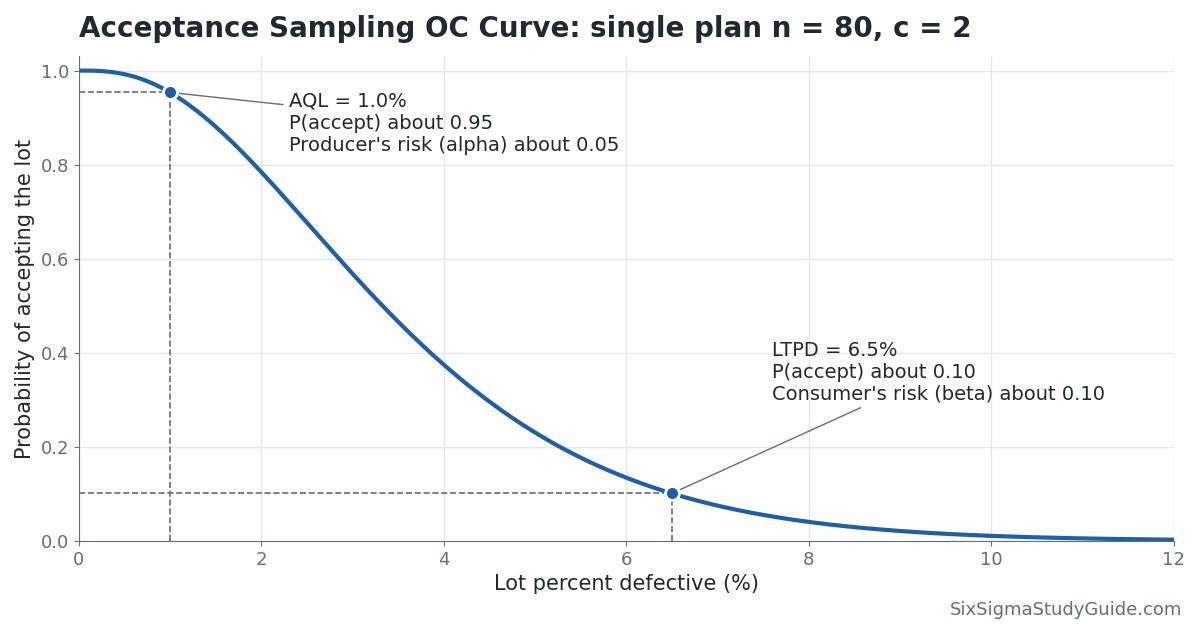
A plan written as “n = 80, c = 2” means: inspect 80 randomly chosen items; accept the lot if you find 0, 1 or 2 defectives; reject it if you find 3 or more. A rejected lot is usually returned to the supplier or screened 100%, with the defectives removed or replaced.

Notice what acceptance sampling does not do. It does not estimate the lot’s quality with any precision, and it does nothing to improve the process that made the lot. It is a sorting decision. Harold Dodge and Harry Romig developed much of the early theory at Bell Telephone Laboratories in the 1920s and 1930s. At the time, buyers had little visibility into how their suppliers’ processes behaved. That context still explains where acceptance sampling fits today.

A Pop-Culture Version: the Bake Off Slice

Watch the judges on The Great British Bake Off. They cut one slice from a cake and pass judgment on the whole bake. That is acceptance sampling with n = 1, and it shows two of its real constraints. The test is destructive, so you cannot “inspect” every slice and still have a cake. And where you cut matters: a slice from the middle can miss an underbaked edge, the same way a sample pulled from the top layer of a pallet can miss the damage at the bottom.

Acceptance Sampling vs 100% Inspection vs SPC

You have three broad ways to deal with the quality of incoming or outgoing product. Each one answers a different question.

ApproachQuestion it answersUse it whenWeakness
Acceptance samplingShould this lot be accepted?Testing is destructive, expensive or slow; lots come from a process you cannot see; you need a defensible, agreed rule with a supplierAccepts some bad lots and rejects some good ones by design; does not improve the process
100% inspectionIs this item good?Lots are small; a defect that escapes is critical (safety, regulatory); the check is cheap or automatedCostly; human inspectors miss defects as fatigue sets in, so even 100% is not 100% effective
SPC (control charts)Is the process stable, and has it changed?You run or can see the process; you want to prevent defects rather than sort themNeeds process access, data discipline and reaction plans; says nothing about a specific lot on its own
Acceptance sampling, 100% inspection and SPC compared. Mature quality systems move from the first two toward the third.

Inspection error matters for both sampling and 100% checks. If your go/no-go gage or your visual inspectors disagree with each other, the plan’s math is built on bad counts. Run a measurement systems analysis, including an attribute agreement study for visual checks, before you trust any accept/reject decision.

Types of Acceptance Sampling Plans

Attributes vs Variables Plans

Attributes plans classify each sampled item as conforming or nonconforming (or count defects per item) and compare the count with an acceptance number. They work for any characteristic you can judge pass/fail, and one plan can cover several characteristics at once. The trade-off is information: a pass/fail result throws away how close each item came to the limit. If you need a refresher on the difference between counting defects and counting defective items, see defects vs defectives.

Variables plans measure a characteristic on a continuous scale (a diameter, a tensile strength), calculate the sample mean and standard deviation, and judge how far the mean sits from the specification limit in standard deviation units. Because each measurement carries more information than a pass/fail result, a variables plan gives the same protection with a smaller sample. The price: it assumes the characteristic is normally distributed, and you need a separate plan for each characteristic you measure.

Single, Double, Multiple and Sequential Sampling

  • Single sampling: one sample of n items, one decision against c. Easiest to train, administer and explain to a supplier.
  • Double sampling: take a first, smaller sample. Very good results accept the lot and very bad results reject it straight away. Results in between trigger a second sample, and the decision uses the combined count. For example: inspect 50; accept on 0 defectives, reject on 3 or more; on 1 or 2, inspect 50 more and accept if the combined total is 3 or fewer. Good lots usually clear on the first sample, so the average amount of inspection drops.
  • Multiple sampling: the same idea extended to several smaller stages.
  • Sequential sampling: inspect one item at a time and, after each, compare the running count with an accept line and a reject line. Keep going while the count sits between them. It comes from Abraham Wald’s sequential probability ratio test and needs the smallest average sample of the four, which makes it attractive for expensive or destructive tests. In exchange, the number of items you might have to inspect is not fixed, which makes scheduling harder.

Single, double and multiple plans can be built to give almost the same protection (nearly the same OC curve). The choice between them is about inspection cost and administrative effort, not about which one is “more accurate”.

AQL, LTPD, Producer’s Risk and Consumer’s Risk

Every sampling plan makes two kinds of mistakes, and the vocabulary of acceptance sampling is built around them. They map directly onto the Type I and Type II errors of hypothesis testing.

TermMeaningTypical value
AQL (acceptable quality level; recent editions of Z1.4 say acceptance quality limit)The worst process average percent defective that is still considered satisfactory. Lots at the AQL should be accepted most of the time.Agreed between buyer and supplier, set separately for each defect class
Producer’s risk (alpha)The probability of rejecting a lot whose quality is at the AQL. The supplier’s risk: a good lot sent back. A Type I error.Around 0.05
LTPD (lot tolerance percent defective), also RQL (rejectable quality level) or LQ (limiting quality)A quality level so poor that lots at it should almost always be rejected.Set by the consumer
Consumer’s risk (beta)The probability of accepting a lot whose quality is at the LTPD. The buyer’s risk: a bad lot let in. A Type II error.Around 0.10
The four numbers that define what an acceptance sampling plan protects against. Alpha is tied to the AQL; beta is tied to the LTPD.

The common misreading, and one of the questions that comes up again and again on quality forums: “We use a 1% AQL, so our lots are at most 1% defective.” No. The AQL describes a process average that the plan will accept most of the time. It is not a cap on any lot. As the worked example below shows, a plan built around a 1% AQL can still accept a 2% defective lot more than three times out of four.

The Operating Characteristic (OC) Curve

The operating characteristic curve is the single most useful picture in acceptance sampling. It plots the probability of accepting a lot (vertical axis) against the lot’s true percent defective (horizontal axis). Every plan has one, and reading it tells you exactly what the plan does.

Acceptance sampling OC curve for the single sampling plan n = 80, c = 2, marking the AQL at 1% and the LTPD at 6.5%
The OC curve for the plan n = 80, c = 2. A lot that is 1% defective (the AQL) is accepted about 95% of the time, so the producer’s risk is about 5%. A lot that is 6.5% defective (the LTPD) is accepted about 10% of the time, which is the consumer’s risk. Everything between those points is a gray zone where the plan’s decision is close to a coin flip.

An ideal plan would draw a vertical cliff: accept every lot better than your limit and reject every lot worse. Only 100% inspection with a perfect inspector can do that. Real OC curves are S-shaped, and the plan’s design decides how steep the slope is.

  • Bigger n makes the curve steeper. More inspection buys better discrimination between good and bad lots.
  • Smaller c (for the same n) shifts the curve left. The plan gets tougher on everyone, including good suppliers, so producer’s risk goes up.
  • Lot size N has surprisingly little effect, as long as the sample is small relative to the lot. Protection comes from the number of items you inspect, not the percentage of the lot.

That last point kills the old “inspect 10% of every lot” habit. With c = 0 and lots that are 2% defective, a 10-piece sample from a lot of 100 accepts about 81% of those lots. A 100-piece sample from a lot of 1,000 accepts about 12%. Same 10%, very different protection.

Worked Example: Building an OC Curve

An injection molder ships connector housings to you in lots of N = 1,000. Your receiving inspection uses a single plan: inspect n = 80 housings for short shots and flash, accept the lot if you find c = 2 or fewer defectives. What happens to a lot that is exactly 1% defective?

Step 1: choose the distribution. Strictly, sampling without replacement from a finite lot follows the hypergeometric distribution. When the sample is no more than about 10% of the lot, the binomial distribution is a close and much easier approximation. Here n/N = 8%, so use the binomial with n = 80 and p = 0.01.

Step 2: add up the accepting outcomes. The lot is accepted if the sample contains 0, 1 or 2 defectives:

  • P(0) = 0.9980 = 0.4475
  • P(1) = 80 x 0.01 x 0.9979 = 0.3616
  • P(2) = 3,160 x 0.012 x 0.9978 = 0.1443 (3,160 is the number of ways to choose 2 items from 80)

P(accept) = 0.4475 + 0.3616 + 0.1443 = 0.953. A lot at 1% defective is accepted about 95% of the time, so the producer’s risk at a 1% AQL is about 0.047.

Step 3: check the exact answer. A 1% defective lot of 1,000 contains exactly 10 defectives. The hypergeometric distribution gives P(0) = 0.4327, P(1) = 0.3800 and P(2) = 0.1481, a total of 0.961. The binomial answer is within one percentage point, which is why the approximation is standard practice.

Step 4: repeat across lot quality. Do the same calculation for other values of p and plot the results. That plot is the OC curve shown above.

The OC Curve Values, Lot by Lot

Lot percent defectiveP(accept), binomialP(accept), hypergeometric (N = 1,000)
0.5%0.9920.996
1%0.9530.961
2%0.7840.789
3%0.5680.564
4%0.3750.365
5%0.2310.219
6.5%0.1010.092
8%0.0400.035
10%0.0110.009
OC curve values for the plan n = 80, c = 2. Calculated with Python (scipy.stats binom and hypergeom) and checked by hand at 1%.

Reading the result. The plan accepts lots at the 1% AQL about 95% of the time and lots at 6.5% about 10% of the time, so the LTPD for a 10% consumer’s risk is about 6.5%. In between, the protection is weak. A 2% lot gets through 78% of the time; a 3% lot, 57%. If a 3% defect rate would hurt your assembly line, this plan does not protect you from it, whatever the AQL says.

AOQ and AOQL in One Paragraph

If rejected lots are screened 100% and every defective is replaced (rectifying inspection), the quality leaving inspection improves. The average outgoing quality (AOQ) for incoming quality p is approximately p x P(accept) x (N – n) / N. AOQ is low when incoming quality is very good (few defectives to begin with) and low when it is very bad (most lots get screened), so it peaks somewhere in the middle. That peak is the average outgoing quality limit (AOQL). For our plan it is about 1.6%, reached when incoming lots are about 2.8% defective. The AOQL is a long-run average, not a guarantee for any single lot.

ANSI/ASQ Z1.4 and Z1.9 Acceptance Sampling Standards

Few people design acceptance sampling plans from scratch. Most use published tables, and in North America that usually means two standards sold by ASQ.

ANSI/ASQ Z1.4 (attributes) is the civilian descendant of the U.S. military’s MIL-STD-105 tables, which were first issued in 1950. When the Department of Defense cancelled MIL-STD-105E in the 1990s, it pointed users to Z1.4. The international counterpart is ISO 2859-1. To use Z1.4 you:

  1. Agree on an AQL for each class of defect (critical, major, minor).
  2. Choose an inspection level. General level II is the default; levels I and III give less or more discrimination; special levels S-1 to S-4 keep samples small for costly or destructive tests.
  3. Look up the sample size code letter from the lot size and inspection level.
  4. Read n and the accept/reject numbers from the table for your code letter, your AQL and the current severity (normal, tightened or reduced).

ANSI/ASQ Z1.9 (variables) is the variables counterpart, derived from MIL-STD-414. It covers single and double specification limits, with methods for when the process standard deviation is known and when it has to be estimated from the sample. It also uses normal, tightened and reduced inspection, and it only applies when the measurements can reasonably be assumed normal. Check that assumption with the data before you rely on the tables.

One point the standards themselves make clear: Z1.4 and Z1.9 are designed for a continuing series of lots, where the switching rules do part of the work. For a single isolated lot, a plan chosen from its OC curve and an LTPD is the better tool.

Switching Rules, Briefly

The switching rules let a sampling scheme react to a supplier’s track record:

  • Normal to tightened: 2 of 5 consecutive lots rejected on original inspection.
  • Tightened back to normal: 5 consecutive lots accepted on original inspection.
  • Normal to reduced: a sustained run of accepted lots (current editions of Z1.4 track this with a switching score), steady production, and approval from the responsible authority.
  • Reduced back to normal: a lot is rejected, production becomes irregular or delayed, or other conditions warrant it.
  • Discontinue: if lots keep failing while on tightened inspection, inspection under the standard stops until the supplier has improved the process.

Skip the switching rules and you lose much of the protection the tables were designed to give. Many companies pick a plan from the normal inspection table and use it forever. That is a common audit finding.

Limitations of Acceptance Sampling: Deming and Others

W. Edwards Deming’s third point for management was to cease dependence on inspection to achieve quality. In Out of the Crisis (1986) he went further and argued that, for a stable process, the minimum total cost comes from one of two extremes: inspect every item or inspect none. His “all-or-none” rule (often called the kp rule) compares the cost of inspecting one item, k1, with the cost of a defective that escapes downstream, k2. If the incoming fraction defective p is below k1/k2, no inspection is cheapest; above it, 100% inspection is cheapest. Sampling sits in between and, in his view, rarely wins. Read more on the Deming page.

Other Practical Objections

Other objections are just as practical:

  • The AQL builds in defects. Agreeing that 1% defective is “acceptable” sits badly with Philip Crosby’s zero defects standard and with continuous improvement generally. Suppliers learn to ship to the AQL.
  • It finds defects after they are made. Shigeo Shingo called this judgment inspection and argued for source inspection and poka-yoke, which stop defects before they happen.
  • It assumes a random sample from a homogeneous lot. Pulling the top layer of a pallet, or mixing two production runs in one lot, quietly breaks the math.
  • It is a weak estimator. Accepting a lot tells you little about its actual quality, and the accept/reject record is a poor substitute for process data. Regulated industries increasingly push back on AQL plans used to validate processes.
  • It adds cost without adding value. Every hour at the receiving bench is an hour spent sorting, which is waste in Lean terms and part of the cost of poor quality.

None of this makes acceptance sampling useless. It makes it a transitional tool: a reasonable defense while you build the supplier relationship and the process evidence that let you inspect less.

Acceptance Sampling in Practice

If you inherit an incoming inspection area, here is how a practitioner works with it.

  1. Draw the OC curve for every plan in use. Most teams know their AQL and have never looked at the LTPD. Showing a manager that the current plan passes a 3% defective lot more than half the time changes the conversation fast.
  2. Classify defects. Critical defects (safety, regulatory) deserve 100% inspection, a c = 0 plan, or better, a process control at the supplier. Do not let them share an AQL with cosmetic defects.
  3. Fix the sampling and the measurement first. Confirm samples are truly random across the lot, and confirm inspectors agree with each other using an attribute agreement study.
  4. Chart the results. Put the fraction defective found in each lot on a p chart by supplier. Lot-by-lot data turns a pile of accept/reject decisions into evidence about the supplier’s process.
  5. Move the control upstream. Ask capable suppliers for control charts and process capability data on the critical characteristics. A supplier with a stable process and a high Cpk earns reduced inspection, skip-lot inspection, or a dock-to-stock arrangement. A supplier who cannot show stability earns tightened inspection and a corrective action request.

Back to the molder in the worked example. If its housings arrive with control charts showing a stable process at 0.2% defective, the receiving bench is spending money to confirm what the supplier’s data already says. If they arrive with no data and lots swing between 0.5% and 4%, the n = 80, c = 2 plan is letting a lot of trouble through. In that case the right fix is a supplier improvement project, not a bigger sample.

Acceptance Sampling Practice Questions

Question 1

A sampling plan inspects n = 50 items from a large lot and accepts the lot only if no defectives are found (c = 0). If the lot is 2% defective, what is the probability the lot is accepted?

(A) 0.02
(B) 0.36
(C) 0.64
(D) 0.98

Answer: (B) 0.36. With a large lot, use the binomial: P(0) = 0.9850 = 0.364. Choice (D) is the chance one item is good, not 50 in a row. The result shows how a c = 0 plan with a modest sample still accepts a 2% defective lot about a third of the time.

Question 2

A lot of 20 printed circuit boards contains 2 defective boards. An inspector selects 5 boards at random without replacement and accepts the lot only if all 5 are good. What is the probability of acceptance?

(A) 0.410
(B) 0.553
(C) 0.590
(D) 0.900

Answer: (B) 0.553. The sample is 25% of a small lot, so use the hypergeometric distribution: P(0) = C(18,5) / C(20,5) = 8,568 / 15,504 = 0.553. Choice (C) is the binomial approximation (0.95 = 0.590), which is noticeably off when the sample is a large share of the lot.

Question 3

On an OC curve, the producer’s risk is best described as:

(A) The probability of accepting a lot at the LTPD
(B) The probability of rejecting a lot at the AQL
(C) The fraction defective at which half of all lots are accepted
(D) The maximum average outgoing quality after rectifying inspection

Answer: (B). Producer’s risk (alpha) is the chance a good lot, one at the AQL, is rejected: 1 minus the probability of acceptance at the AQL. (A) is the consumer’s risk (beta), (C) is sometimes called the indifference quality level, and (D) is the AOQL.

Acceptance Sampling FAQ

Does a 1% AQL mean my lots are at most 1% defective?

No. It means the plan will accept lots at 1% defective most of the time, typically about 95%. Worse lots are accepted too, at a rate you can read from the OC curve. If you need to keep out lots at a particular defect level, design the plan around the LTPD.

Can I use AQL sampling for in-process inspection?

You can, but it is usually the wrong tool. Inside your own process you can see the process, so a control chart tells you more, sooner, and points you toward the cause. Lot sentencing makes most sense at a hand-off between organizations or departments.

Why doesn’t the sample size grow in proportion to the lot size?

Because the protection depends on how many items you inspect, not on what fraction of the lot they represent. Z1.4 does increase n with lot size, but slowly, mainly because a wrong decision on a big lot costs more.

Is acceptance sampling on the Six Sigma Green Belt or Black Belt exam?

It is not listed as its own topic in the current ASQ Green Belt or Black Belt bodies of knowledge, or in the IASSC outlines. It is a core topic for ASQ’s Certified Quality Engineer exam. For Green and Black Belt candidates, the tested skills underneath it (binomial and hypergeometric probability, alpha and beta risk) are well worth practicing this way.

When you’re ready, there are a few ways I can help:

First, join 12,000+ other Six Sigma professionals by subscribing to my email newsletter. A short read every Monday to start your work week off correctly. Always free.

* * *

If you’re looking to pass your Six Sigma Yellow Belt, Green Belt or Black Belt exam, I’d recommend starting with my affordable study guide:

1)→ 🟡Pass Your Six Sigma Yellow Belt: built for ASQ, IASSC and ILSSI, 1,700+ practice questions with explanations, and six full-length mock exams for your exam

2)→ 🟢Pass Your Six Sigma Green Belt: a study guide organized by the exam Body of Knowledge, 1,300+ practice questions with detailed answer explanations, and 20 full-length mock exams

3)→ ⚫Pass Your Six Sigma Black Belt: the full Black Belt Body of Knowledge, 2,200+ practice questions with detailed answer explanations, and 20 full-length mock exams

You’ve spent so much effort learning Lean Six Sigma. Why leave passing your certification exam up to chance? This comprehensive study guide offers 1,700+ exam-like questions for Yellow Belts, 1,300+ for Green Belts and 2,200+ for Black Belts with full answer walkthroughs, access to instructors, detailed study material, and more.

​ Thousands have used this system to prepare. Join them here. 

Control Chart Rules: Western Electric and Nelson Rules for Spotting Out of Control Signals

Control chart rules are the tests that tell you when a point, or a pattern of points, is unlikely enough to come from common-cause variation that you should go looking for a special cause. One point beyond the control limits is the rule everyone knows. The others look for runs, trends and clusters that stay inside the limits but still signal that the process has changed.

The trouble is that different books, software packages and even different pages on the same site quote different numbers: seven points in a row, eight, nine. This page sets out the two classic rule sets, the Western Electric rules and the Nelson rules, explains where the numbers differ and why, and states one rule set to use. It also covers the part most articles skip: every rule you add makes the chart more sensitive and also raises the false alarm rate.

The Short Answer: Five Core Control Chart Rules

If you want one set to remember, use these five. They are the four Western Electric zone rules plus the six-point trend rule from Lloyd Nelson’s list, and they are the rules shown in our control charts study guide.

RuleSignalUsually means
1One point beyond a control limit (more than 3 sigma from the center line)A large, sudden change or a one-off event
24 out of 5 consecutive points beyond 1 sigma, on the same sideA smaller shift in the mean
32 out of 3 consecutive points beyond 2 sigma, on the same sideA medium shift in the mean
48 consecutive points on the same side of the center lineA sustained small shift
56 consecutive points steadily increasing or decreasingA drift: tool wear, heating, fatigue
The five core control chart rules used on SixSigmaStudyGuide.com. Rules 1 to 4 are the four Western Electric rules (1956), with its rules 2 and 3 swapped to match our study guide chart. Rule 5 is Nelson’s test 3 (1984).

For an exam, read the numbers in the question. If a question says “seven points in a row”, it is using a different rule set, and the question’s numbers win. The sections below explain where those other numbers come from.

Control Chart Zones A, B and C

Most run rules are written in terms of zones. Divide each half of the chart, between the center line and a control limit, into three bands one standard deviation wide:

  • Zone C: within 1 sigma of the center line. About 68% of points fall here when the process is stable.
  • Zone B: between 1 and 2 sigma. About 27% of points.
  • Zone A: between 2 and 3 sigma. About 4% of points.
  • Beyond the limits: more than 3 sigma away. About 0.27% of points, roughly 1 in 370.

Those percentages assume the plotted values are close to normally distributed and independent of each other. That is a reasonable assumption for subgroup averages on an X-bar chart, less so for individual values or ranges. Here, “sigma” means the standard deviation of whatever is plotted. On an X-bar chart that is the standard error of the subgroup mean, not the standard deviation of individual parts.

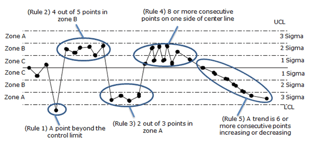
Control chart rules shown on a chart divided into zones A, B and C
The five core rules on a zoned chart: a point beyond the limit, 4 of 5 points in zone B or beyond, 2 of 3 points in zone A, 8 or more points on one side of the center line, and a trend of 6 points.

The Western Electric Rules

The Western Electric Company published its Statistical Quality Control Handbook in 1956 to teach shop-floor people how to read Shewhart charts. Its four zone tests became the first widely used set of control chart rules. Each test looks at one half of the chart at a time.

Western Electric ruleTest (one side of the center line)
1Any single point beyond 3 sigma (zone A or beyond)
22 out of 3 consecutive points beyond 2 sigma (in zone A or beyond)
34 out of 5 consecutive points beyond 1 sigma (in zone B or beyond)
48 consecutive points on the same side of the center line (zone C or beyond)
The four Western Electric zone rules (Western Electric, Statistical Quality Control Handbook, 1956).

The handbook also describes other unnatural patterns, such as trends, cycles, stratification and mixtures, but it treats those as patterns to recognize rather than as fixed counting rules.

Our five core rules use the same four tests in a different order, to match our study guide chart. Core rule 2 is Western Electric rule 3 (4 out of 5 beyond 1 sigma). Core rule 3 is Western Electric rule 2 (2 out of 3 beyond 2 sigma). On an exam, go by the pattern, not the number.

The Nelson Rules

In 1984 Lloyd S. Nelson published eight “tests for special causes” in the Journal of Quality Technology. They include the Western Electric zone tests, change the run length, and add tests for trends, oscillation and the patterns that bad subgrouping produces. Minitab and several other packages number their tests the same way, so these are the rules most learners meet in software.

Nelson testPatternWhat it points to
11 point beyond 3 sigmaA large shift, a one-off event or a recording error
29 points in a row on the same side of the center lineA sustained shift in the mean
36 points in a row steadily increasing or decreasingA drift
414 points in a row alternating up and downTwo sources used alternately (two machines, two operators, two suppliers) or over-adjustment
52 out of 3 points beyond 2 sigma, same sideA medium shift
64 out of 5 points beyond 1 sigma, same sideA small shift
715 points in a row within 1 sigma, either sideStratification: subgroups that mix sources, so the limits are too wide
88 points in a row beyond 1 sigma, either side, none within 1 sigmaA mixture of two processes, with points avoiding the middle
Nelson’s eight tests for special causes (Nelson, 1984). Test 5 is our core rule 3 and test 6 is our core rule 2 (Western Electric rules 2 and 3).

Nelson also gave advice on how to use them. Apply tests 1 to 4 routinely. Add tests 5 and 6 when the cost of a late signal justifies a few more false alarms. Treat tests 7 and 8 as diagnostics for how the subgroups were formed, which is the subject of rational subgrouping.

Why the Numbers Differ: Seven, Eight or Nine Points?

The run rule is where sources disagree most. Western Electric uses 8 points on one side. Nelson uses 9, and he chose it deliberately: a run of 9 has a false alarm probability close to that of a single point beyond 3 sigma, so every test carries about the same weight. Older texts such as Grant and Leavenworth used 7, and many company procedures and some SPC software still do.

The arithmetic shows why the choice matters. If points are independent and the process is centered, each point has a 50% chance of falling above the center line. The chance that a given run of points all fall on one particular side is 0.5 raised to that many points. Counting either side doubles it:

Run on one sideProbability for a stable, centered process
7 points2 × 0.57 = 1 in 64
8 points2 × 0.58 = 1 in 128
9 points2 × 0.59 = 1 in 256
One point beyond 3 sigma (for comparison)0.0027, about 1 in 370
Each extra point in the run halves the chance of a false run signal.

None of these numbers is wrong. They are different points on the same trade-off between catching small shifts early and crying wolf. What is wrong is mixing them, which is why this site uses one stated set.

Run charts are a separate case. A run chart has no control limits, so its rules count points around the median instead of the mean and use different thresholds. One widely used set in healthcare improvement (Perla, Provost and Murray, 2011) calls 6 or more points on one side of the median a shift and 5 or more points steadily up or down a trend. Don’t carry run chart numbers onto a control chart, or the reverse.

The False Alarm Trade-Off of Adding Control Chart Rules

Every rule is a small hypothesis test, and every test has a Type I error rate. Run several tests on every point and the chance that at least one fires by accident adds up. This is the same alpha and beta trade-off covered in errors in hypothesis testing, applied to a chart.

The standard way to measure it is the average run length (ARL): how many points you plot, on average, before the chart signals. When the process is stable you want a long ARL (few false alarms). After a real shift you want a short one (fast detection).

Rules appliedAverage points to a false alarm (stable process)Average points to detect a 1-sigma shift in the mean
Rule 1 only (point beyond 3 sigma)37044
Nelson tests 1 to 4about 120about 17
Western Electric rules 1 to 4about 92about 9
Five core rules (this site)about 77about 9
All eight Nelson testsabout 73about 10
Average run lengths for normally distributed, independent points. Rule 1 values are exact; Western Electric’s 92 matches Champ and Woodall’s exact 91.75 (1987); the other rows are from a 20,000-run simulation by SixSigmaStudyGuide.com and are approximate.

Read the table from left to right. Adding zone rules cuts the time to catch a 1-sigma shift from about 44 points to about 9, which is a big gain. The price is a false alarm roughly every 77 to 92 points instead of every 370, about four times as many. Piling on further rules after that buys almost no extra sensitivity for this kind of shift, but it keeps adding false alarms.

Scale it to a plant. Run 50 charts and plot one point on each per day, and the five core rules will produce a false alarm somewhere roughly every day and a half. That’s manageable if the reaction plan is “look, log, and only adjust when you find a cause”. It’s a disaster if every signal triggers a process adjustment, because adjusting a stable process adds variation. The quincunx shows why.

Sports fans know the trap from the other side. In 1985 Gilovich, Vallone and Tversky argued that basketball’s “hot hand” streaks were mostly what chance produces anyway. Later work by Miller and Sanjurjo (2018) found a subtle bias in that analysis, and the debate about how real the hot hand is continues. The lesson for control charts holds either way: random data produce streaks more often than intuition expects. Run rules exist to put a number on “unusual” so that people stop reacting to streaks that chance alone explains.

Which Rules to Use, and When

  • Setting up limits (Phase I). When you first calculate limits from historical data, use rule 1 and the run rules to find and remove the subgroups with assignable causes. Then recalculate.
  • Routine monitoring (Phase II) on X-bar and individuals charts. Use the five core rules. They catch shifts of about 1 sigma or more within roughly ten points.
  • Range, S and attribute charts. These plot statistics with skewed distributions, so the zone percentages above don’t hold and zone rules give more false alarms on one side than the other. Lean on rule 1 and the run and trend rules, and check what your software does by default.
  • Small, slow drifts matter more than false alarms. If you need to catch shifts smaller than 1 sigma, adding more rules is a poor tool. Use a CUSUM chart or an EWMA chart instead.
  • Autocorrelated data. Chemical processes, temperatures and anything measured very frequently often have points that depend on the previous point. Run rules assume independence and will fire constantly. Fix the sampling interval or model the autocorrelation first.

Whatever you choose, write it into the SPC procedure and the reaction plan, so that everyone reading the chart applies the same rules.

Apply the Control Chart Rules by Hand: a 12-Point Exercise

Here are twelve consecutive subgroup averages, expressed as the number of sigma units above (positive) or below (negative) the center line. Decide which of the five core rules fire, and at which point, before reading the answer.

Point123456789101112
Sigma units+0.3-0.8+1.2+1.5+1.1+1.8+0.9+2.4+2.2+0.5-0.2+3.3
ZoneCCBBBBCAACCbeyond
Twelve subgroup averages in sigma units from the center line, with their zones.

Answer. Rule 2 fires at point 6: of points 2 to 6, four (1.2, 1.5, 1.1, 1.8) are beyond 1 sigma on the high side. The process has probably shifted up a little, and it did so around point 3. Rule 3 fires at point 9: two of the last three points (2.4 and 2.2) are beyond 2 sigma on the high side. Rule 4 fires at point 10: points 3 to 10 are eight in a row above the center line. Rule 1 fires at point 12: 3.3 is beyond the upper control limit. Rule 5 never fires; there is no run of six steadily increasing or decreasing values. Notice the order. The zone rules caught the shift at point 6, six points before the first point went outside the limits. That is the case for using them.

Example: Control Chart Rules on an Injection Molding Line

A molder charts the weight of a part on an X-bar and R chart, five consecutive shots every hour. Here is how a month of signals might read, and what each one sent the team to check.

  1. Two of three hourly averages beyond 2 sigma, above the center line (rule 3). The timing matched a new lot of resin. The lot’s melt flow was at the high end of its specification. The team logged it and asked the supplier for tighter lot-to-lot control.
  2. Six averages in a row, each heavier than the last (rule 5). A drifting thermocouple was letting the barrel run a little hotter each hour. Maintenance replaced it before any part went out of specification. That is the payoff of run rules: the problem was caught while every point was still inside the limits.
  3. Fourteen averages alternating high and low (Nelson test 4). The cause wasn’t the process at all. Two technicians were taking the hourly sample, one from cavity 1 and one from cavity 2. The fix was a sampling instruction: always the same cavity, or a separate chart per cavity.
  4. Fifteen averages in a row, all within 1 sigma (Nelson test 7). After a well-meant change, each subgroup contained one shot from each of the mold’s four cavities. Cavity-to-cavity differences inflated the ranges and widened the limits, so the chart looked calm and could no longer detect anything. See rational subgrouping for the fix.

Notice that two of the four signals were caused by how the data were collected, not by the process. That is common in real work. When a rule fires, check the measurement and the sampling before you touch the machine.

What to Do When a Control Chart Rule Fires

  1. Mark the point and note which rule fired. The rule hints at the kind of cause: a sudden event (rule 1), a shift (rules 2 to 4), a drift (rule 5) or a sampling problem (Nelson tests 4, 7 and 8).
  2. Check the data first: a typo, a wrong gage, a different sampler, a changed sampling method.
  3. Look for what changed at that time: material lot, shift, setup, maintenance, environment. A run rule fires at the end of the run, so the cause usually started at its beginning.
  4. Act on the cause, not the point. If you find a cause, fix it and record it. If you don’t, log the signal and keep watching. Don’t adjust the process just to move the next point.
  5. Recalculate limits only when the process has really changed, for example after a confirmed improvement, never just to make signals go away.

Control Chart Rules FAQ

What are the 8 control chart rules?

Usually this means Nelson’s eight tests: 1 point beyond 3 sigma; 9 in a row on one side; 6 in a row increasing or decreasing; 14 alternating up and down; 2 of 3 beyond 2 sigma; 4 of 5 beyond 1 sigma; 15 in a row within 1 sigma; 8 in a row beyond 1 sigma on either side. Some study materials list eight rules with slightly different counts, so check the source.

What is the difference between the Western Electric and Nelson rules?

Western Electric (1956) has four zone rules with an 8-point run. Nelson (1984) keeps the zone tests, lengthens the run to 9 points, and adds tests for trends, alternation, stratification and mixtures, for eight in total.

What is the rule of seven?

A simplified run rule: seven consecutive points on one side of the center line, or seven in a row trending up or down, signal a non-random pattern. It appears in older quality texts and in project management study materials. A stable, centered process produces a 7-point run on one side about once in 64 tries, which is why stricter rule sets use 8 or 9.

Does one point outside the limits always mean the process is out of control?

It means there is strong evidence of a special cause, strong enough to investigate. About 1 point in 370 from a stable process will fall outside 3-sigma limits by chance, so a single point with no cause found is possible. Two in a short time is much stronger evidence.

Should I turn on every rule in my SPC software?

Usually not. Each extra rule adds false alarms, and the table above shows most of the sensitivity comes from the first few. Turn on the rules your reaction plan can actually handle, and use the subgrouping tests (Nelson 7 and 8) when you are checking how a chart was set up.

Are control chart rules on the Six Sigma exam?

Yes. ASQ’s Black Belt body of knowledge asks you to “interpret control charts and distinguish between common and special causes using rules for determining statistical control” (VIII.A.5). The Green Belt body of knowledge covers distinguishing common and special causes from control chart analysis (VI.A.1), and ILSSI’s Green Belt list includes tests for special cause variation. Expect a sketch or a list of points and a question about which rule, if any, is broken. If you want exam-style practice on reading charts, Pass Your Six Sigma Green Belt includes control chart questions with full walkthroughs.

When you’re ready, there are a few ways I can help:

First, join 12,000+ other Six Sigma professionals by subscribing to my email newsletter. A short read every Monday to start your work week off correctly. Always free.

* * *

If you’re looking to pass your Six Sigma Yellow Belt, Green Belt or Black Belt exam, I’d recommend starting with my affordable study guide:

1)→ 🟡Pass Your Six Sigma Yellow Belt: built for ASQ, IASSC and ILSSI, 1,700+ practice questions with explanations, and six full-length mock exams for your exam

2)→ 🟢Pass Your Six Sigma Green Belt: a study guide organized by the exam Body of Knowledge, 1,300+ practice questions with detailed answer explanations, and 20 full-length mock exams

3)→ ⚫Pass Your Six Sigma Black Belt: the full Black Belt Body of Knowledge, 2,200+ practice questions with detailed answer explanations, and 20 full-length mock exams

You’ve spent so much effort learning Lean Six Sigma. Why leave passing your certification exam up to chance? This comprehensive study guide offers 1,700+ exam-like questions for Yellow Belts, 1,300+ for Green Belts and 2,200+ for Black Belts with full answer walkthroughs, access to instructors, detailed study material, and more.

​ Thousands have used this system to prepare. Join them here. 

Do You Need Minitab for Six Sigma? Minitab vs Excel vs Calculator

Do you need Minitab for Six Sigma? To pass the exam, no. You cannot use it in the exam room anyway. To run real projects, you need some statistics software, and Excel can carry you further than most people think.

This page answers the three questions students ask me most about tools. First, what can I bring into the exam? Second, which calculator should I use? Third, can I do the statistics in Excel or by hand?

What you can bring into the exam, by certifying body

Rules change. I checked each body’s own pages in October 2026. Confirm with your body before exam day.

BodyOpen or closed bookCalculatorSoftware (Minitab, Excel)
ASQ (test center or remote)Open book. All references, including notes, must be bound and stay bound. Hand-stapled pages and loose notes are not allowed.An on-screen basic scientific calculator is built into every computer-based exam. At a test center you may bring a silent, hand-held, battery-operated calculator with no programmable memory. ASQ names the TI-89 as not allowed.No.
IASSCClosed book. IASSC gives you its own Reference Document as a download at the start of the exam. Do not bring your own copy.A non-programmable four-function or scientific calculator. IASSC lists the SHARP EL 501XBWH, TI-34, TI-30X and Casio FX-115 as examples. Graphing and programmable models (TI-83, TI-84, Casio FX9750, FX5800P) are not allowed. Neither are phone calculators.No. IASSC names Minitab and SigmaXL as not permitted.
VillanovaOpen book. Villanova confirmed to us in October 2026 that you may use course materials, notes and other resources.Not published. Check with Villanova.Not published. Check with Villanova.
ILSSIOpen book. ILSSI confirmed to us in October 2026 that printed materials, notes or a PDF of the course materials are allowed.Not published. Check with ILSSI.Not published. Check with ILSSI.

Sources: ASQ’s Six Sigma Black Belt certification page (the same rules appear on the Green and Yellow Belt pages) and its remote proctoring FAQ; IASSC’s permitted resources and open book answers; Villanova’s certification requirements; ILSSI’s certification page.

ASQ remote exams have extra rules

If you take an ASQ exam at home through remote proctoring, three things change.

  • No scratch paper and no pens. You use the Scratchpad inside the exam software instead. Practice your math without paper at least once before the day.
  • Your references still have to be bound.
  • ASQ’s FAQ allows “built-in calculators” and asks you to show your references and calculator at check-in. It does not say plainly whether a hand-held calculator is fine at home. If you want to use one, ask ASQ before exam day.

IASSC: learn the reference document before the exam

IASSC exams are closed book, but you are not on your own. The IASSC Reference Document holds the formulas and tables you get on screen. IASSC links to it from its permitted resources page. Download it now and study with it, so you know where everything sits when the clock is running.

Which calculator should you use for the Six Sigma exam?

Use a plain, non-programmable scientific calculator. ASQ and IASSC both allow one, and it does everything the exam needs.

Then make sure it has these keys, and that you can find them without looking:

  • ln and e^x for rolled throughput yield, Poisson and exponential questions
  • x^y and √ for NPV, binomial and standard deviation work
  • x² and memory keys (M+, MR) for sums of squares
  • Σ or statistics mode, if your body allows it, for mean and standard deviation. Check that your model is non-programmable.

Buy it early. Do every practice exam with it. The middle of the exam is a bad time to learn where the inverse key is.

I used an HP 10bII (HP sells the current model as the 10bII+) for my ASQ Six Sigma Black Belt exam. It is a financial calculator with no programming mode, no graphing and no text storage, so it fits ASQ’s rule. It has the statistics keys (mean and standard deviation) and NPV and IRR built in, which saves time on the project selection questions. A plain scientific model works too: IASSC names the TI-30X and the Casio FX-115 as examples, and both meet ASQ’s rule. Check any other model against ASQ’s rule before you buy it. (Here is how I studied and passed.) For the rest of your exam bag, see what to bring to an open-book ASQ exam.

Do you need Minitab to pass the Six Sigma exam?

No. No certifying body above lets you use Minitab or any other software in the exam. The exam tests whether you can pick the right tool, run the numbers with a formula, a table and a calculator, and read the result.

What you do need:

  • The formulas. Get my free Six Sigma Formula Reference Sheet from the ASQ Green Belt or ASQ Black Belt study guide page. Members of the Pass Your Six Sigma Green Belt and Black Belt courses also get my Black Belt Formula Sheet PDF in the course downloads: the business and process metrics the statistics sheets skip (NPV, DPMO to sigma level, RTY, takt time, OEE and the distributions), each with a worked example.
  • The tables: z, t, chi-square and F. Learn to read each one. Our Z table guide explains the two common z table layouts.
  • Practice reading results. Exam-style questions can show an ANOVA table or a regression printout and ask what it means. Learn what each column is.
  • Knowing which test to use. The Hypothesis Tests Study Guide lays out the choices.

Software helps you study in one way: you can check your hand calculations. Run a practice problem by hand, then in Excel. If the answers match, you understand it.

Do you need Minitab for Six Sigma projects?

For real projects, you need some statistics software. Real data sets are too big for a calculator. Many Six Sigma courses teach with Minitab. If your employer has a license, use it. Minitab offers a free trial.

If you do not have a license, these options cost little or nothing:

ToolCostGood forLimits
Excel with the Analysis ToolPakIncluded with desktop Excel (Windows and Mac). You switch it on as an add-in.t-tests, F-test, one- and two-way ANOVA, regression, correlation, descriptive statistics, histogramsNo control charts, capability, Gage R&R or DOE menus. You build those from formulas.
Real Statistics Resource Pack for ExcelFree downloadAdds many tests the ToolPak lacks, including more ANOVA and regression options and non-parametric testsAn add-in written by one author; check its version against your Excel version.
JASPFree, open sourcePoint-and-click statistics with a Quality Control module: control charts, process capability, Gage R&R and other measurement system studies, DOE worksheetsA separate program, not Excel. Some menus are named differently from Minitab.
RFree, open sourceAnything, if you are willing to write code. The qcc package covers control charts and capability.A learning curve. Best if you or your team already code.

Commercial Excel add-ins built for Six Sigma also exist. SigmaXL is one; IASSC names it in its rules. Compare price and features against what your projects need.

To turn on the Analysis ToolPak in Excel for Windows: File, Options, Add-ins, choose Excel Add-ins in the Manage box, click Go, tick Analysis ToolPak. On a Mac: Tools, Excel Add-ins. Microsoft’s Analysis ToolPak guide lists every tool. Once it is on, look for Data Analysis on the Data tab.

Free templates for Pareto charts, box plots and more are on our Six Sigma Excel templates page.

How to run the main Six Sigma tests in Excel or by hand

Each row shows the Excel route and the by-hand formula. The by-hand version is what the exam tests.

TestIn ExcelBy hand (exam)Learn it
One-sample t-testNo ToolPak tool. Compute t yourself, then p = T.DIST.2T(ABS(t), n-1)t = (x̄ – μ₀) / (s / √n), df = n – 1, compare to the t tableOne sample t test
Two-sample t-testToolPak: t-Test: Two-Sample Assuming Equal Variances (or Unequal). Or =T.TEST(A, B, 2, 2) for equal variances, type 3 for unequalPooled: t = (x̄₁ – x̄₂) / (s_p √(1/n₁ + 1/n₂))Two sample t tests
Paired t-testToolPak: t-Test: Paired Two Sample for Means. Or =T.TEST(A, B, 2, 1)t = d̄ / (s_d / √n) on the differencesPaired t test
F-test for two variancesToolPak: F-Test Two-Sample for Variances. =F.TEST(A, B) gives a two-tailed pF = s₁² / s₂² (larger on top), compare to the F tableF-test
One-way ANOVAToolPak: Anova: Single Factor. Two-factor versions are there tooF = MS between / MS within, from the sums of squares tableANOVA
Chi-square test of independenceNo ToolPak tool. Build the expected table (row total x column total / grand total), then =CHISQ.TEST(observed, expected) gives pχ² = Σ (O – E)² / E, df = (rows – 1)(columns – 1)Chi-square test of independence
Simple linear regressionToolPak: Regression (gives the ANOVA table, R², coefficients and p-values). Or =SLOPE, =INTERCEPT, =RSQ, =LINESTb₁ = Sxy / Sxx, b₀ = ȳ – b₁x̄Linear regression
Control limits (I-MR)No built-in chart. Compute the mean, the moving ranges and their average, then the limits with the formulasUCL/LCL = x̄ ± 2.66 x MR̄; UCL for the MR chart = 3.267 x MR̄I-MR chart
Control limits (X-bar R)Same approach with the subgroup means and rangesx̿ ± A₂R̄; R chart: D₃R̄ to D₄R̄ (constants from the table for your subgroup size)X-bar R charts
Cp and Cpk=(USL-LSL)/(6*s) and =MIN(USL-mean, mean-LSL)/(3*s). Use the within-subgroup sigma (R̄/d₂) for Cp and Cpk; =STDEV.S of all the data gives Pp and PpkSame formulasProcess capability (Cp and Cpk)
Normal probabilities=NORM.S.DIST(z, TRUE) for the area to the left; =NORM.S.INV(p) for the reversez = (x – μ) / σ and the z tableZ scores and the z table

Worked example: a two-sample t-test both ways

Two lines, five cycle times each (minutes).

  • Line A: 12, 14, 11, 13, 15. Mean 13.0. Standard deviation 1.581.
  • Line B: 15, 17, 16, 14, 18. Mean 16.0. Standard deviation 1.581.

By hand. The standard deviations are equal, so the pooled s_p is 1.581. The standard error is 1.581 x √(1/5 + 1/5) = 1.581 x 0.632 = 1.000. So t = (13.0 – 16.0) / 1.000 = -3.00. With 8 degrees of freedom, the two-tailed critical t at α = 0.05 is 2.306. Since |t| = 3.00 is bigger than 2.306, reject the null. The lines differ.

In Excel. Put A in A2:A6 and B in B2:B6. =T.TEST(A2:A6, B2:B6, 2, 2) returns 0.017. Below 0.05. Same conclusion.

Worked example: I-MR control limits by hand

Eight readings: 10.2, 9.8, 10.5, 10.1, 9.9, 10.4, 10.0, 10.3.

  • Mean = 81.2 / 8 = 10.15
  • Moving ranges: 0.4, 0.7, 0.4, 0.2, 0.5, 0.4, 0.3. Average MR̄ = 2.9 / 7 = 0.414
  • Individuals chart: UCL = 10.15 + 2.66 x 0.414 = 11.25. LCL = 10.15 – 2.66 x 0.414 = 9.05
  • Moving range chart: UCL = 3.267 x 0.414 = 1.35. LCL = 0.

In Excel, the same numbers come from =AVERAGE, =ABS(B3-B2) filled down, and the two formulas. Add a line chart and draw the limits as extra series. That is an I-MR chart without Minitab.

Worked example: chi-square by hand

A survey asks 100 people two yes/no questions. The counts are 30 and 20 in the first row, 20 and 30 in the second. Every expected count is 50 x 50 / 100 = 25. Each cell adds (5)² / 25 = 1, so χ² = 4.0. The critical value at α = 0.05 with 1 degree of freedom is 3.841. Reject independence. In Excel, =CHISQ.TEST on the observed and expected tables returns 0.046.

The short version

  • Exam: a non-programmable scientific calculator, the formulas, the tables, and practice reading output. No Minitab.
  • Projects: Minitab if your employer has it. Otherwise Excel with the Analysis ToolPak, plus JASP or R for control charts and capability.
  • Rules: check your body’s current page before exam day. They change.

If arithmetic is the part that worries you, the Math Confidence for Six Sigma course starts from square roots, powers and lookup tables.

External resources

When you’re ready, there are a few ways I can help:

First, join 12,000+ other Six Sigma professionals by subscribing to my email newsletter. A short read every Monday to start your work week off correctly. Always free.

* * *

If you’re looking to pass your Six Sigma Yellow Belt, Green Belt or Black Belt exam, I’d recommend starting with my affordable study guide:

1)→ 🟡Pass Your Six Sigma Yellow Belt: built for ASQ, IASSC and ILSSI, 1,700+ practice questions with explanations, and six full-length mock exams for your exam

2)→ 🟢Pass Your Six Sigma Green Belt: a study guide organized by the exam Body of Knowledge, 1,300+ practice questions with detailed answer explanations, and 20 full-length mock exams

3)→ ⚫Pass Your Six Sigma Black Belt: the full Black Belt Body of Knowledge, 2,200+ practice questions with detailed answer explanations, and 20 full-length mock exams

You’ve spent so much effort learning Lean Six Sigma. Why leave passing your certification exam up to chance? This comprehensive study guide offers 1,700+ exam-like questions for Yellow Belts, 1,300+ for Green Belts and 2,200+ for Black Belts with full answer walkthroughs, access to instructors, detailed study material, and more.

​ Thousands have used this system to prepare. Join them here.