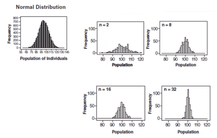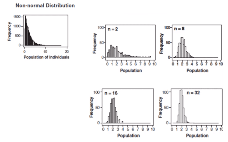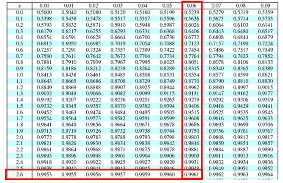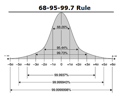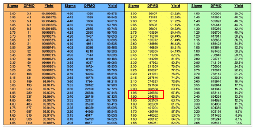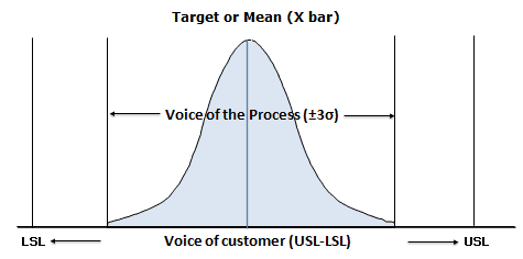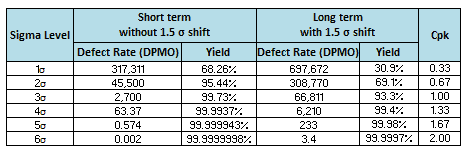

A Histogram is a bar graph that shows the frequency with which data occurs within a certain interval. In other words, it is a bar chart showing the number of times an outcome is repeated. In Six Sigma, we can use a histogram to visualize what is going on. It can reflect the voice of the process.
A Histogram is a popular statistical method for showing a visual model of a continuous series or a class interval frequency distribution. A bar graph is used for categorical data.
Why Use a Histogram?
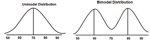
A histogram is one of the 7 Quality tools that are often used to assess process behavior and demonstrate if the data follows a normal distribution. The purpose of a histogram is to graphically summarize the distribution of a univariate data set. It shows the center, the spread, the skewness of the data, the presence of outliers, and the presence of multiple modes in the data.
While a normal histogram tells you information about the data, a properly made histogram tells you more than the raw data. A normal histogram helps you understand the normal distribution, dispersion, and central tendencies of the data. In contrast, a great histogram helps to visualize the VOC. In addition, you can include the specification limits to reflect the needs of the customer.
When to use a Histogram
Six Sigma uses histograms when the data is numerical and continuous. Histograms are used to view the overall traits of the data distribution and peaks of the distribution in the data set. Furthermore, it can be used to identify whether the distribution is skewed or symmetric and to show the outliers. Histograms help to determine if the process meets the needs of the customer, and it also helps to identify the process changes over time.
Differences between frequency distributions and Histogram
A frequency distribution is the table: it sorts raw data, also known as observations, into classes and counts how many fall in each, often with tally marks or check marks. A histogram is the bar graph of that table. Each class gets one bar, and the bar height is the count or relative frequency.
How to analyze the Histogram
Six Sigma users can apply the pattern seen in the histogram to discern a process variation. It is a frequency distribution graph in which the class interval is plotted on the X- axis and their respective frequencies on the Y- axis. It is a two-dimensional diagram.
- The width of each bar displays the interval size
- The height of each bar displays the frequency of the interval
- There are no gaps between bars that are next to one another
- Continuous nature of quantitative data
The height or length of each rectangle shows the frequency of the class, and the breadth shows the size of the class interval. Therefore, the total area covered by the histogram represents the total number of times the data point occurs.
Different shapes of Histogram
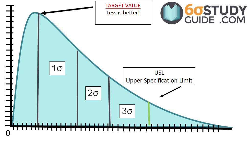
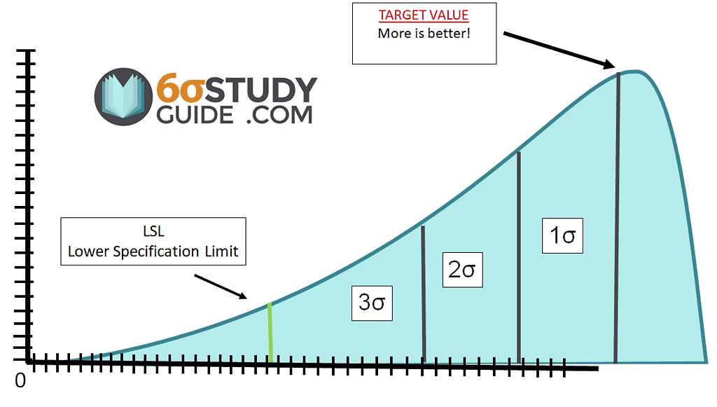
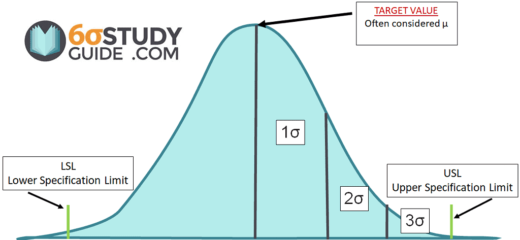
When reading a histogram, we want to ask: How many peaks are there? Are there any outliers in the data? Does it look near symmetrical and bell-shaped?
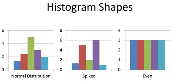
Bell-Shaped :
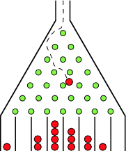
If there is a bell shape, your data may be normally distributed. That does not mean no variation. It suggests common cause variation, with no obvious special cause or mixed source (such as one of the 6Ms).
Spiked
If there are multiple spikes in the chart, there is likely variation in the process.
Even
On the other hand, if all of the bars are at the same level, we are not likely correctly measuring the process.
Doing statistical analysis usually includes the following:
- Measuring the central tendency.
- Measuring the variation.
Steps to Create a Histogram
The construction of a histogram starts with the division of a frequency distribution into equal classes, and each class is a vertical bar. It is used to plot data density, especially continuous data like weight or height.
- Collect the data
- Arrange the data points in order and assign categories
- Find the lowest and highest value
- Find the number of intervals
- Use 2^k = N where k = # of categories (smallest positive integer) and N = # of data.
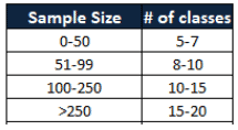
- Compute the intervals with covering the entire range of the data set
- Find the frequency of occurrence for each of the data points as per the interval
- Draw the bar chart preserving counts and categories
Example
Ex. Delay times in minutes for an airline
1) Get Data
Use continuous data– data collection from a frequency distribution check sheet.
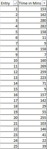
Step 2: Order it and Assign Categories
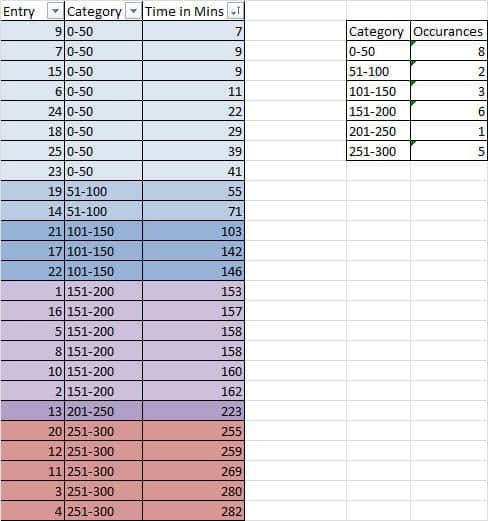
- Note: The number of cells (columns) affects the shape – so choose wisely!
- Could use 2^k = N where k = # of categories (smallest positive integer) and N = # of data.
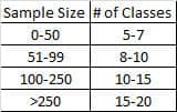
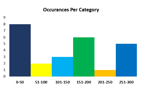
Step 3: Create a Bar Chart Preserving Counts and Categories
Advantages
- You can visualize the distribution of the data.
- It summarizes the large data set graphically.
- It helps to make future decisions based on data.
- You can use it to assist in decision making.
- Simple to understand and also easy to communicate with the team.
Disadvantages
- It uses only continuous data.
- More difficult to compare two data sets.
- Difficult to read values because data is grouped into data sets.
How to Create a Histogram in Minitab
Useful Videos
When you’re ready, there are a few ways I can help:
First, join 12,000+ other Six Sigma professionals by subscribing to my email newsletter. A short read every Monday to start your work week off correctly. Always free.
* * *
If you’re looking to pass your Six Sigma Yellow Belt, Green Belt or Black Belt exam, I’d recommend starting with my affordable study guide:
1)→ 🟡Pass Your Six Sigma Yellow Belt: built for ASQ, IASSC and ILSSI, 1,700+ practice questions with explanations, and six full-length mock exams for your exam
2)→ 🟢Pass Your Six Sigma Green Belt: a study guide organized by the exam Body of Knowledge, 1,300+ practice questions with detailed answer explanations, and 20 full-length mock exams
3)→ ⚫Pass Your Six Sigma Black Belt: the full Black Belt Body of Knowledge, 2,200+ practice questions with detailed answer explanations, and 20 full-length mock exams
You’ve spent so much effort learning Lean Six Sigma. Why leave passing your certification exam up to chance? This comprehensive study guide offers 1,700+ exam-like questions for Yellow Belts, 1,300+ for Green Belts and 2,200+ for Black Belts with full answer walkthroughs, access to instructors, detailed study material, and more.
Thousands have used this system to prepare. Join them here.