

Acceptance sampling is the decision rule a receiving dock, a final inspection station or a customer uses to accept or reject a whole lot of product based on a sample drawn from it. You inspect a few items, count what you find, and the count tells you what to do with the other few thousand.
It sounds simple, and the arithmetic is simple. The hard part is understanding what a sampling plan actually protects you against, and what it quietly lets through. This guide covers the plans, the vocabulary (AQL, LTPD, producer’s risk, consumer’s risk), the operating characteristic curve with a worked example, the ANSI/ASQ Z1.4 and Z1.9 standards, and the limits that led Deming and others to argue you should depend on it as little as possible.
A note on exams first. Acceptance sampling is a core topic in ASQ’s Certified Quality Engineer (CQE) body of knowledge. The current ASQ Green Belt and Black Belt bodies of knowledge, and the IASSC outlines, do not list it as its own topic. It still shows up in Green Belt and Black Belt work, because it sits right next to topics they do test: the binomial and hypergeometric distributions, Type I and Type II errors, and the choice between inspection and statistical process control.
What Is Acceptance Sampling?
A sampling plan has three pieces:
- The lot: a batch of N items made under the same conditions, such as one shipment of 1,000 molded housings.
- The sample size, n: how many items you draw at random and inspect.
- The acceptance number, c: the most defectives you can find in the sample and still accept the lot. Find c or fewer, accept. Find more than c, reject.
A plan written as “n = 80, c = 2” means: inspect 80 randomly chosen items; accept the lot if you find 0, 1 or 2 defectives; reject it if you find 3 or more. A rejected lot is usually returned to the supplier or screened 100%, with the defectives removed or replaced.
Notice what acceptance sampling does not do. It does not estimate the lot’s quality with any precision, and it does nothing to improve the process that made the lot. It is a sorting decision. Harold Dodge and Harry Romig developed much of the early theory at Bell Telephone Laboratories in the 1920s and 1930s, at a time when buyers had little visibility into how their suppliers’ processes behaved. That context still explains where acceptance sampling fits today.
A Pop-Culture Version: the Bake Off Slice
Watch the judges on The Great British Bake Off. They cut one slice from a cake and pass judgment on the whole bake. That is acceptance sampling with n = 1, and it shows two of its real constraints. The test is destructive, so you cannot “inspect” every slice and still have a cake. And where you cut matters: a slice from the middle can miss an underbaked edge, the same way a sample pulled from the top layer of a pallet can miss the damage at the bottom.
Acceptance Sampling vs 100% Inspection vs SPC
You have three broad ways to deal with the quality of incoming or outgoing product. Each one answers a different question.
| Approach | Question it answers | Use it when | Weakness |
|---|---|---|---|
| Acceptance sampling | Should this lot be accepted? | Testing is destructive, expensive or slow; lots come from a process you cannot see; you need a defensible, agreed rule with a supplier | Accepts some bad lots and rejects some good ones by design; does not improve the process |
| 100% inspection | Is this item good? | Lots are small; a defect that escapes is critical (safety, regulatory); the check is cheap or automated | Costly; human inspectors miss defects as fatigue sets in, so even 100% is not 100% effective |
| SPC (control charts) | Is the process stable, and has it changed? | You run or can see the process; you want to prevent defects rather than sort them | Needs process access, data discipline and reaction plans; says nothing about a specific lot on its own |
Inspection error matters for both sampling and 100% checks. If your go/no-go gage or your visual inspectors disagree with each other, the plan’s math is built on bad counts. Run a measurement systems analysis, including an attribute agreement study for visual checks, before you trust any accept/reject decision.
Types of Acceptance Sampling Plans
Attributes vs Variables Plans
Attributes plans classify each sampled item as conforming or nonconforming (or count defects per item) and compare the count with an acceptance number. They work for any characteristic you can judge pass/fail, and one plan can cover several characteristics at once. The trade-off is information: a pass/fail result throws away how close each item came to the limit. If you need a refresher on the difference between counting defects and counting defective items, see defects vs defectives.
Variables plans measure a characteristic on a continuous scale (a diameter, a tensile strength), calculate the sample mean and standard deviation, and judge how far the mean sits from the specification limit in standard deviation units. Because each measurement carries more information than a pass/fail result, a variables plan gives the same protection with a smaller sample. The price: it assumes the characteristic is normally distributed, and you need a separate plan for each characteristic you measure.
Single, Double, Multiple and Sequential Sampling
- Single sampling: one sample of n items, one decision against c. Easiest to train, administer and explain to a supplier.
- Double sampling: take a first, smaller sample. Very good results accept the lot and very bad results reject it straight away. Results in between trigger a second sample, and the decision uses the combined count. For example: inspect 50; accept on 0 defectives, reject on 3 or more; on 1 or 2, inspect 50 more and accept if the combined total is 3 or fewer. Good lots usually clear on the first sample, so the average amount of inspection drops.
- Multiple sampling: the same idea extended to several smaller stages.
- Sequential sampling: inspect one item at a time and, after each, compare the running count with an accept line and a reject line. Keep going while the count sits between them. It comes from Abraham Wald’s sequential probability ratio test and needs the smallest average sample of the four, which makes it attractive for expensive or destructive tests. In exchange, the number of items you might have to inspect is not fixed, which makes scheduling harder.
Single, double and multiple plans can be built to give almost the same protection (nearly the same OC curve). The choice between them is about inspection cost and administrative effort, not about which one is “more accurate”.
AQL, LTPD, Producer’s Risk and Consumer’s Risk
Every sampling plan makes two kinds of mistakes, and the vocabulary of acceptance sampling is built around them. They map directly onto the Type I and Type II errors of hypothesis testing.
| Term | Meaning | Typical value |
|---|---|---|
| AQL (acceptable quality level; recent editions of Z1.4 say acceptance quality limit) | The worst process average percent defective that is still considered satisfactory. Lots at the AQL should be accepted most of the time. | Agreed between buyer and supplier, set separately for each defect class |
| Producer’s risk (alpha) | The probability of rejecting a lot whose quality is at the AQL. The supplier’s risk: a good lot sent back. A Type I error. | Around 0.05 |
| LTPD (lot tolerance percent defective), also RQL (rejectable quality level) or LQ (limiting quality) | A quality level so poor that lots at it should almost always be rejected. | Set by the consumer |
| Consumer’s risk (beta) | The probability of accepting a lot whose quality is at the LTPD. The buyer’s risk: a bad lot let in. A Type II error. | Around 0.10 |
The common misreading, and one of the questions that comes up again and again on quality forums: “We use a 1% AQL, so our lots are at most 1% defective.” No. The AQL describes a process average that the plan will accept most of the time. It is not a cap on any lot. As the worked example below shows, a plan built around a 1% AQL can still accept a 2% defective lot more than three times out of four.
The Operating Characteristic (OC) Curve
The operating characteristic curve is the single most useful picture in acceptance sampling. It plots the probability of accepting a lot (vertical axis) against the lot’s true percent defective (horizontal axis). Every plan has one, and reading it tells you exactly what the plan does.
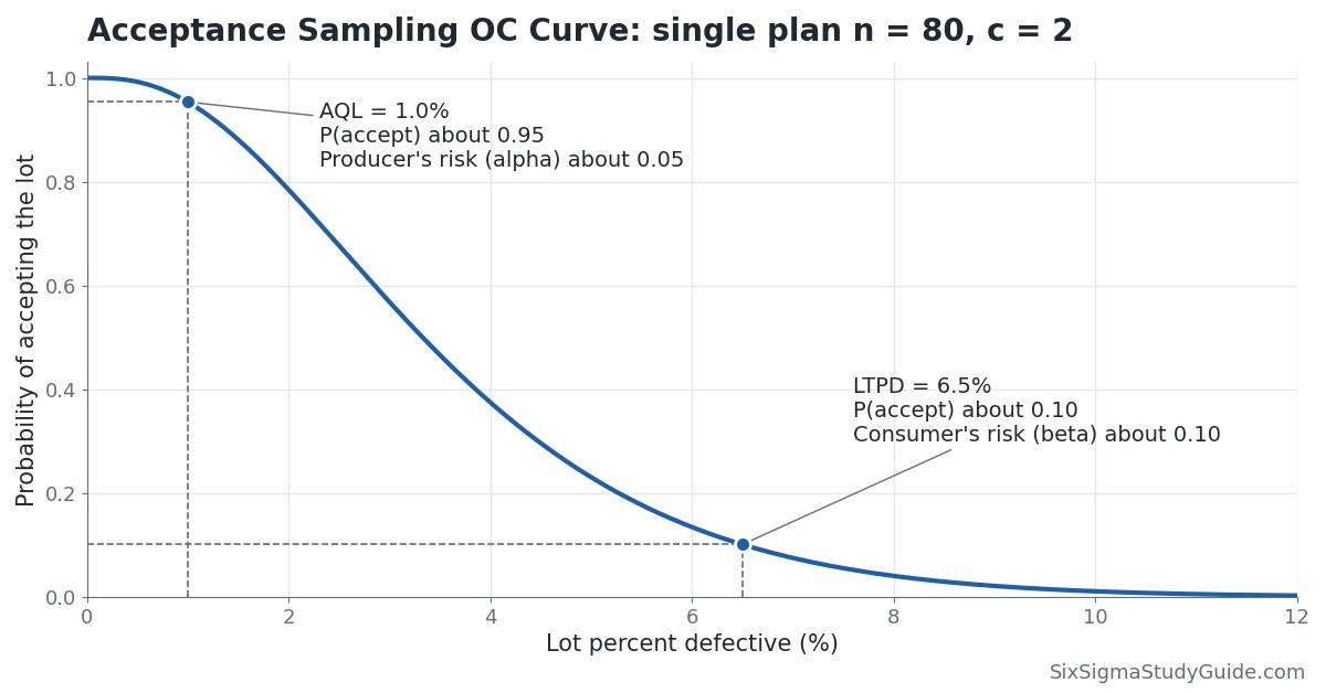
An ideal plan would draw a vertical cliff: accept every lot better than your limit and reject every lot worse. Only 100% inspection with a perfect inspector can do that. Real OC curves are S-shaped, and the plan’s design decides how steep the slope is.
- Bigger n makes the curve steeper. More inspection buys better discrimination between good and bad lots.
- Smaller c (for the same n) shifts the curve left. The plan gets tougher on everyone, including good suppliers, so producer’s risk goes up.
- Lot size N has surprisingly little effect, as long as the sample is small relative to the lot. Protection comes from the number of items you inspect, not the percentage of the lot.
That last point kills the old “inspect 10% of every lot” habit. With c = 0 and lots that are 2% defective, a 10-piece sample from a lot of 100 accepts about 81% of those lots. A 100-piece sample from a lot of 1,000 accepts about 12%. Same 10%, very different protection.
Worked Example: Building an OC Curve
An injection molder ships connector housings to you in lots of N = 1,000. Your receiving inspection uses a single plan: inspect n = 80 housings for short shots and flash, accept the lot if you find c = 2 or fewer defectives. What happens to a lot that is exactly 1% defective?
Step 1: choose the distribution. Strictly, sampling without replacement from a finite lot follows the hypergeometric distribution. When the sample is no more than about 10% of the lot, the binomial distribution is a close and much easier approximation. Here n/N = 8%, so use the binomial with n = 80 and p = 0.01.
Step 2: add up the accepting outcomes. The lot is accepted if the sample contains 0, 1 or 2 defectives:
- P(0) = 0.9980 = 0.4475
- P(1) = 80 x 0.01 x 0.9979 = 0.3616
- P(2) = 3,160 x 0.012 x 0.9978 = 0.1443 (3,160 is the number of ways to choose 2 items from 80)
P(accept) = 0.4475 + 0.3616 + 0.1443 = 0.953. A lot at 1% defective is accepted about 95% of the time, so the producer’s risk at a 1% AQL is about 0.047.
Step 3: check the exact answer. A 1% defective lot of 1,000 contains exactly 10 defectives. The hypergeometric distribution gives P(0) = 0.4327, P(1) = 0.3800 and P(2) = 0.1481, a total of 0.961. The binomial answer is within one percentage point, which is why the approximation is standard practice.
Step 4: repeat across lot quality. Do the same calculation for other values of p and plot the results. That plot is the OC curve shown above.
| Lot percent defective | P(accept), binomial | P(accept), hypergeometric (N = 1,000) |
|---|---|---|
| 0.5% | 0.992 | 0.996 |
| 1% | 0.953 | 0.961 |
| 2% | 0.784 | 0.789 |
| 3% | 0.568 | 0.564 |
| 4% | 0.375 | 0.365 |
| 5% | 0.231 | 0.219 |
| 6.5% | 0.101 | 0.092 |
| 8% | 0.040 | 0.035 |
| 10% | 0.011 | 0.009 |
Reading the result. The plan accepts lots at the 1% AQL about 95% of the time and lots at 6.5% about 10% of the time, so the LTPD for a 10% consumer’s risk is about 6.5%. In between, the protection is weak. A 2% lot gets through 78% of the time; a 3% lot, 57%. If a 3% defect rate would hurt your assembly line, this plan does not protect you from it, whatever the AQL says.
AOQ and AOQL in One Paragraph
If rejected lots are screened 100% and every defective is replaced (rectifying inspection), the quality leaving inspection improves. The average outgoing quality (AOQ) for incoming quality p is approximately p x P(accept) x (N – n) / N. AOQ is low when incoming quality is very good (few defectives to begin with) and low when it is very bad (most lots get screened), so it peaks somewhere in the middle. That peak is the average outgoing quality limit (AOQL). For our plan it is about 1.6%, reached when incoming lots are about 2.8% defective. The AOQL is a long-run average, not a guarantee for any single lot.
ANSI/ASQ Z1.4 and Z1.9 Acceptance Sampling Standards
Few people design acceptance sampling plans from scratch. Most use published tables, and in North America that usually means two standards sold by ASQ.
ANSI/ASQ Z1.4 (attributes) is the civilian descendant of the U.S. military’s MIL-STD-105 tables, which were first issued in 1950. When the Department of Defense cancelled MIL-STD-105E in the 1990s, it pointed users to Z1.4. The international counterpart is ISO 2859-1. To use Z1.4 you:
- Agree on an AQL for each class of defect (critical, major, minor).
- Choose an inspection level. General level II is the default; levels I and III give less or more discrimination; special levels S-1 to S-4 keep samples small for costly or destructive tests.
- Look up the sample size code letter from the lot size and inspection level.
- Read n and the accept/reject numbers from the table for your code letter, your AQL and the current severity (normal, tightened or reduced).
ANSI/ASQ Z1.9 (variables) is the variables counterpart, derived from MIL-STD-414. It covers single and double specification limits, with methods for when the process standard deviation is known and when it has to be estimated from the sample. It also uses normal, tightened and reduced inspection, and it only applies when the measurements can reasonably be assumed normal. Check that assumption with the data before you rely on the tables.
One point the standards themselves make clear: Z1.4 and Z1.9 are designed for a continuing series of lots, where the switching rules do part of the work. For a single isolated lot, a plan chosen from its OC curve and an LTPD is the better tool.
Switching Rules, Briefly
The switching rules let a sampling scheme react to a supplier’s track record:
- Normal to tightened: 2 of 5 consecutive lots rejected on original inspection.
- Tightened back to normal: 5 consecutive lots accepted on original inspection.
- Normal to reduced: a sustained run of accepted lots (current editions of Z1.4 track this with a switching score), steady production, and approval from the responsible authority.
- Reduced back to normal: a lot is rejected, production becomes irregular or delayed, or other conditions warrant it.
- Discontinue: if lots keep failing while on tightened inspection, inspection under the standard stops until the supplier has improved the process.
Skip the switching rules and you lose much of the protection the tables were designed to give. Many companies pick a plan from the normal inspection table and use it forever. That is a common audit finding.
Limitations of Acceptance Sampling: Deming and Others
W. Edwards Deming’s third point for management was to cease dependence on inspection to achieve quality. In Out of the Crisis (1986) he went further and argued that, for a stable process, the minimum total cost comes from one of two extremes: inspect every item or inspect none. His “all-or-none” rule (often called the kp rule) compares the cost of inspecting one item, k1, with the cost of a defective that escapes downstream, k2. If the incoming fraction defective p is below k1/k2, no inspection is cheapest; above it, 100% inspection is cheapest. Sampling sits in between and, in his view, rarely wins. Read more on the Deming page.
Other objections are just as practical:
- The AQL builds in defects. Agreeing that 1% defective is “acceptable” sits badly with Philip Crosby’s zero defects standard and with continuous improvement generally. Suppliers learn to ship to the AQL.
- It finds defects after they are made. Shigeo Shingo called this judgment inspection and argued for source inspection and poka-yoke, which stop defects before they happen.
- It assumes a random sample from a homogeneous lot. Pulling the top layer of a pallet, or mixing two production runs in one lot, quietly breaks the math.
- It is a weak estimator. Accepting a lot tells you little about its actual quality, and the accept/reject record is a poor substitute for process data. Regulated industries increasingly push back on AQL plans used to validate processes.
- It adds cost without adding value. Every hour at the receiving bench is an hour spent sorting, which is waste in Lean terms and part of the cost of poor quality.
None of this makes acceptance sampling useless. It makes it a transitional tool: a reasonable defense while you build the supplier relationship and the process evidence that let you inspect less.
Acceptance Sampling in Practice
If you inherit an incoming inspection area, here is how a practitioner works with it.
- Draw the OC curve for every plan in use. Most teams know their AQL and have never looked at the LTPD. Showing a manager that the current plan passes a 3% defective lot more than half the time changes the conversation fast.
- Classify defects. Critical defects (safety, regulatory) deserve 100% inspection, a c = 0 plan, or better, a process control at the supplier. Do not let them share an AQL with cosmetic defects.
- Fix the sampling and the measurement first. Confirm samples are truly random across the lot, and confirm inspectors agree with each other using an attribute agreement study.
- Chart the results. Put the fraction defective found in each lot on a p chart by supplier. Lot-by-lot data turns a pile of accept/reject decisions into evidence about the supplier’s process.
- Move the control upstream. Ask capable suppliers for control charts and process capability data on the critical characteristics. A supplier with a stable process and a high Cpk earns reduced inspection, skip-lot inspection, or a dock-to-stock arrangement. A supplier who cannot show stability earns tightened inspection and a corrective action request.
Back to the molder in the worked example. If its housings arrive with control charts showing a stable process at 0.2% defective, the receiving bench is spending money to confirm what the supplier’s data already says. If they arrive with no data and lots swing between 0.5% and 4%, the n = 80, c = 2 plan is letting a lot of trouble through, and the right fix is a supplier improvement project rather than a bigger sample.
Acceptance Sampling Practice Questions
Question 1
A sampling plan inspects n = 50 items from a large lot and accepts the lot only if no defectives are found (c = 0). If the lot is 2% defective, what is the probability the lot is accepted?
(A) 0.02
(B) 0.36
(C) 0.64
(D) 0.98
Answer: (B) 0.36. With a large lot, use the binomial: P(0) = 0.9850 = 0.364. Choice (D) is the chance one item is good, not 50 in a row. The result shows how a c = 0 plan with a modest sample still accepts a 2% defective lot about a third of the time.
Question 2
A lot of 20 printed circuit boards contains 2 defective boards. An inspector selects 5 boards at random without replacement and accepts the lot only if all 5 are good. What is the probability of acceptance?
(A) 0.410
(B) 0.553
(C) 0.590
(D) 0.900
Answer: (B) 0.553. The sample is 25% of a small lot, so use the hypergeometric distribution: P(0) = C(18,5) / C(20,5) = 8,568 / 15,504 = 0.553. Choice (C) is the binomial approximation (0.95 = 0.590), which is noticeably off when the sample is a large share of the lot.
Question 3
On an OC curve, the producer’s risk is best described as:
(A) The probability of accepting a lot at the LTPD
(B) The probability of rejecting a lot at the AQL
(C) The fraction defective at which half of all lots are accepted
(D) The maximum average outgoing quality after rectifying inspection
Answer: (B). Producer’s risk (alpha) is the chance a good lot, one at the AQL, is rejected: 1 minus the probability of acceptance at the AQL. (A) is the consumer’s risk (beta), (C) is sometimes called the indifference quality level, and (D) is the AOQL.
Acceptance Sampling FAQ
Does a 1% AQL mean my lots are at most 1% defective?
No. It means the plan will accept lots at 1% defective most of the time, typically about 95%. Worse lots are accepted too, at a rate you can read from the OC curve. If you need to keep out lots at a particular defect level, design the plan around the LTPD.
Can I use AQL sampling for in-process inspection?
You can, but it is usually the wrong tool. Inside your own process you can see the process, so a control chart tells you more, sooner, and points you toward the cause. Lot sentencing makes most sense at a hand-off between organizations or departments.
Why doesn’t the sample size grow in proportion to the lot size?
Because the protection depends on how many items you inspect, not on what fraction of the lot they represent. Z1.4 does increase n with lot size, but slowly, mainly because a wrong decision on a big lot costs more.
Is acceptance sampling on the Six Sigma Green Belt or Black Belt exam?
It is not listed as its own topic in the current ASQ Green Belt or Black Belt bodies of knowledge, or in the IASSC outlines. It is a core topic for ASQ’s Certified Quality Engineer exam. For Green and Black Belt candidates, the tested skills underneath it (binomial and hypergeometric probability, alpha and beta risk) are well worth practicing this way.
Related Pages
- Binomial distribution and hypergeometric distribution
- Errors in hypothesis testing (alpha and beta)
- Statistical process control (SPC) and the control charts study guide
- Process capability (Cp and Cpk)
- Measurement systems analysis (MSA)
When you’re ready, there are a few ways I can help:
First, join 12,000+ other Six Sigma professionals by subscribing to my email newsletter. A short read every Monday to start your work week off correctly. Always free.
* * *
If you’re looking to pass your Six Sigma Green Belt or Black Belt exams, I’d recommend starting with my affordable study guide:
1)→ 🟢Pass Your Six Sigma Green Belt: a study guide organized by the exam Body of Knowledge, 1,000+ practice questions with detailed answer explanations, and 15+ full-length mock exams
2)→ ⚫Pass Your Six Sigma Black Belt: the full Black Belt Body of Knowledge, 2,000+ practice questions with detailed answer explanations, and 15+ full-length mock exams
You’ve spent so much effort learning Lean Six Sigma. Why leave passing your certification exam up to chance? This comprehensive study guide offers 1,000+ exam-like questions for Green Belts (2,000+ for Black Belts) with full answer walkthroughs, access to instructors, detailed study material, and more.
Thousands have used this system to prepare. Join them here.