
Standard deviation is used to measure the amount of variation in a process. This is one of the most common measures of variability in a data set or population.
There are 2 types of equations: Sample and Population.
What is the difference between Population and Sample?
Population refers to ALL of a set, and the sample is a subset. We most often have a sample and are trying to infer something about the whole group. However, if we want to know a truth of a subset of a whole population, use the Population equation.
Use Population When:
- You have the entire population.
- You have a larger population sample, but you are only interested in this sample and do not wish to generalize your findings to the population.
Use Sample When (Most often):
- If all you have is a sample but wish to make a statement about the population standard deviation from which the sample is drawn, you need to use the sample SD.
Remember: It is impossible to have a negative standard deviation.
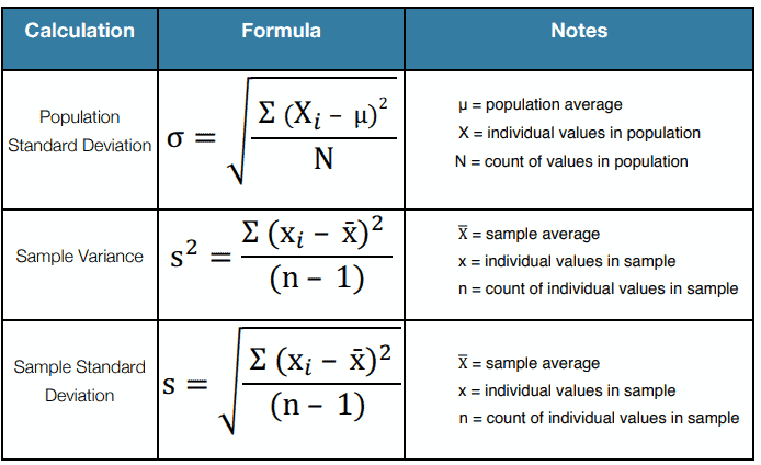
Population standard deviation: σ = √[ Σ(Xi – μ)2 / N ]. Here μ is the population average, Xi is each value in the population and N is the count of values in the population.
Sample variance: s2 = Σ(xi – x̄)2 / (n – 1). Here x̄ is the sample average, xi is each value in the sample and n is the count of values in the sample.
Sample standard deviation: s = √[ Σ(xi – x̄)2 / (n – 1) ], the square root of the sample variance.
How to Measure the Standard Deviation for a Sample (s)
Standard Deviation for a Sample (s)
- Calculate the mean of the data set (x-bar)
- Subtract the mean from each value in the data set
- Square the differences found in step 2.
- Add up the squared differences found in step 3.
- Divide the total from step 4 by (n – 1) for sample data
- (Note: At this point, you have the variance of the data).
- Take the square root of the result from step 5 to get the SD
Example of Standard Deviation for a Sample (s)
The length of 8 bars in centimeters is 9, 12, 13, 11, 12, 8, 10, and 11. Calculate the sample standard deviation of the length of the bar.
- Calculate the mean of the data set
(9+12+13+11+12+8+10+11)/8=86/8=10.75
2. Subtract the mean from each value in the data set
- 9-10.75=-1.75
- 12-10.75=1.25
- 13-10.75=2.25
- 11-10.75=0.25
- 12-10.75=1.25
- 8-10.75=-2.75
- 10-10.75=-0.75
- 11-10.75=0.25
3. Square the differences found in step 2.
- (-1.75)2 =3.06
- (1.25)2 =1.56
- (2.25)2 =5.06
- (0.25)2 =0.06
- (1.25)2 =1.56
- (-2.75)2 =7.56
- (-0.75)2 =0.56
- (0.25)2 =0.06
4. Add up the squared differences found in step 3 =19.50
5. Divide the total from step 4 by (n – 1) for sample data = 19.5/(8 – 1) = 2.79, so the variance is 2.79
6. Take the square root of the result from step 5, SD of sample bar length = 1.67
How to Measure the Standard Deviation for a Population (σ)
Standard Deviation for a Population (σ)
- Calculate the mean of the data set (μ)
- Subtract the mean from each value in the data set
- Square the differences found in step 2.
- Add up the squared differences found in step 3.
- Divide the total from step 4 by N (for population data).
- (Note: At this point, you have the variance of the data).
- Take the square root of the result from step 5 to get the SD
Example: Sample Standard Deviation of Egg Weights (s)
Nana’s Bakery wants to optimize the consistency of its cakes. The recipe calls for a certain number of eggs. The problem is that there is variation in egg sizes. Six eggs were randomly selected, and the following weights were recorded (measured in ounces).
2.25; 1.75; 2.0; 2.5; 2.3; 1.8
What is the sample standard deviation (s) of the egg weights? The six eggs are a random sample, so divide by n – 1.
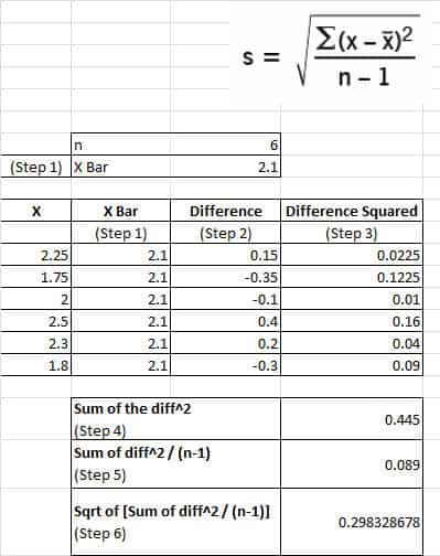
Step 1: mean x̄ = (2.25 + 1.75 + 2.0 + 2.5 + 2.3 + 1.8) / 6 = 12.6 / 6 = 2.1
Steps 2 and 3: subtract the mean from each weight, then square each difference.
| x (oz) | x – x̄ | (x – x̄)2 |
|---|---|---|
| 2.25 | 0.15 | 0.0225 |
| 1.75 | -0.35 | 0.1225 |
| 2.0 | -0.10 | 0.0100 |
| 2.5 | 0.40 | 0.1600 |
| 2.3 | 0.20 | 0.0400 |
| 1.8 | -0.30 | 0.0900 |
| Sum | 0 | 0.445 |
Step 4: sum of the squared differences = 0.445
Step 5: sample variance s2 = 0.445 / (6 – 1) = 0.089
Step 6: s = √0.089 = 0.2983 oz
Standard Deviation and Variance
Variance is Std Dev ^2.
Std Dev = Sqrt(variance)
The Uniform Distribution
A uniform distribution is a continuous probability distribution. It describes the condition where all possible outcomes of a random experiment are equally likely to occur. For the uniform distribution, the probability density function f(x) is constant over the possible values of x.
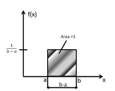
The density is a flat rectangle from a to b. Its width is b – a and its height is 1 / (b – a), so the total area is 1.
The formula for Mean and standard deviation of uniform distribution
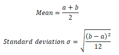
Mean = (a + b) / 2
Standard deviation σ = √[ (b – a)2 / 12 ]
Probability density function
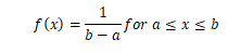
f(x) = 1 / (b – a) for a ≤ x ≤ b
The Area between p and q

P(p < x < q) = base × height = (q – p) × 1 / (b – a)
Area right of x
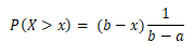
P(X > x) = (b – x) × 1 / (b – a)
Area left of x
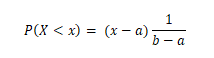
P(X < x) = (x – a) × 1 / (b – a)
Example: Daily sales revenue at Beta stores is uniformly distributed between $6,000 and $20,000. Find:
- Mean
- Standard deviation
- Probability that daily revenue falls between $10,000 and $12,000
- Probability that daily revenue is at least $16,000
Revenue is a continuous variable, so the continuous uniform model fits. A count, such as the number of phones sold, is discrete and would use the discrete uniform formulas instead.
Let X be the daily revenue in dollars. X follows the uniform distribution over (6,000, 20,000), so the probability density function is f(x) = 1 / (20,000 − 6,000) = 1/14,000 for 6,000 ≤ x ≤ 20,000.
- Mean = (a + b) / 2 = (6,000 + 20,000) / 2 = $13,000
- Standard deviation σ = √[(b − a)² / 12] = √[(14,000)² / 12] = 14,000 / √12 ≈ $4,041
- P(10,000 < X < 12,000) = (12,000 − 10,000) × 1/14,000 = 1/7 ≈ 0.143
- P(X ≥ 16,000) = (20,000 − 16,000) × 1/14,000 = 2/7 ≈ 0.286
Walkthrough: Standard Deviation of a Sample Proportion
Question: In a factory, 5% of manufactured bolts are known to be defective. A quality inspector randomly samples 400 bolts. What is the standard deviation of the sample proportion of defective bolts, assuming the distribution is approximately normal?
Step 1: Identify the known values
- Population proportion (
p) = 0.05 - Sample size (
n) = 400
Step 2: Use the standard deviation formula for a sample proportion
σp̂ = √[ p(1 − p) / n ]
Step 3: Plug in the values
σp̂ = √[ 0.05 × (1 − 0.05) / 400 ]
= √[ 0.05 × 0.95 / 400 ]
= √[ 0.0475 / 400 ]
= √0.00011875
Step 4: Calculate
√0.00011875 ≈ 0.0109
Final Answer:
The standard deviation of the sample proportion of defective bolts is approximately 0.0109.
Helpful Videos
Video on Variance
The Normal Curve
The Uniform Distribution
When you’re ready, there are a few ways I can help:
First, join 12,000+ other Six Sigma professionals by subscribing to my email newsletter. A short read every Monday to start your work week off correctly. Always free.
* * *
If you’re looking to pass your Six Sigma Yellow Belt, Green Belt or Black Belt exam, I’d recommend starting with my affordable study guide:
1)→ 🟡Pass Your Six Sigma Yellow Belt: built for ASQ, IASSC and ILSSI, 1,700+ practice questions with explanations, and six full-length mock exams for your exam
2)→ 🟢Pass Your Six Sigma Green Belt: a study guide organized by the exam Body of Knowledge, 1,300+ practice questions with detailed answer explanations, and 20 full-length mock exams
3)→ ⚫Pass Your Six Sigma Black Belt: the full Black Belt Body of Knowledge, 2,200+ practice questions with detailed answer explanations, and 20 full-length mock exams
You’ve spent so much effort learning Lean Six Sigma. Why leave passing your certification exam up to chance? This comprehensive study guide offers 1,700+ exam-like questions for Yellow Belts, 1,300+ for Green Belts and 2,200+ for Black Belts with full answer walkthroughs, access to instructors, detailed study material, and more.
Thousands have used this system to prepare. Join them here.