
How Do You Know if a Process Is Following a Normal Distribution?

Many of the analysis required in the Green Belt and Black Belt Body of knowledge assumes a normal distribution. There’s a good reason for this; normal distributions have a nice, symmetrical shape that makes working with them much easier (like in an ANOVA, for example!) But how do you know if your process is following a normal distribution? Use these tests to find out.

Visual Normality Tests / Graphical Analysis

  • Visual examination. Make a histogram or another bar graph. Only reject normality in the presence of “gross non-normality”, extreme departures from symmetry.
  • If you see a bell curve, a distribution is approaching normal.
  • Tall, thin curve = smaller standard deviation.
  • Fatter, lower curve = larger standard deviation.
  • You can test using a Normal Probability Plot. The probability plot transforms the data into a normal distribution and plots it as a scatter diagram.
    • Normal data will follow the trend line.
    • Non-normal data will have more points farther from the trend line.
  • The peak of the normal curve is an indication of the average, which is the center of process variation. An average of a group of numbers is an indication of the central tendency.

Quantifiable Normality Tests

  • Use the Chi Square Goodness of Fit test.
  • Follow the Anderson-Darling Normality test or Critical Value Method.
    • The output includes the Anderson-Darling statistic, A-squared, and both a p-value and critical values for A-squared.
    • “Null hypothesis” is that the data is normal. The “alternative hypothesis” is that the data is non-normal. Reject the Null hypothesis (i.e., accept the alternative) when p<=alpha or A-squared>critical value.
    • if p > alpha then the data is normal.
    • if A-squared < Critical Value, then the data is normal
  • Mean is the inverse of the Poisson distribution.
  • The smaller the standard deviation, the tighter the grouping of data around the mean.

Worked Example

Say you have 30 cycle-time measurements and want to know if they’re normal enough to run an ANOVA. Plot them on a normal probability plot: if the points hug the straight trend line with only minor scatter at the very ends, treat the data as normal and proceed. If a chunk of points curves noticeably away from the line, especially in the middle of the range rather than just the tails, that’s a sign of real non-normality, not just sampling noise. Follow up with the Anderson-Darling test for a formal yes/no answer: if the p-value comes back above your alpha (typically 0.05), you don’t have enough evidence to call the data non-normal, so it’s reasonable to treat it as normal for the analysis you’re about to run.

A Batting Average Example

Batting averages across a full league tend to cluster into a bell shape: a handful of exceptional hitters at one extreme, a handful of struggling ones at the other, and most players somewhere in the thick middle. That’s the visual, intuitive version of what a histogram or probability plot is checking for: are the extreme values rare compared to the common middle, the way they should be if the process generating them is well-behaved?

What If It’s Not Normal?

Confirming non-normality isn’t the end of the analysis, it’s a fork in the road. Options include a Box-Cox transformation to make the data approximately normal, switching to a non-parametric test that doesn’t assume normality in the first place, or checking whether the non-normality itself is meaningful (a bimodal distribution, for instance, often means you’re actually looking at two different processes mixed together, which is itself a useful finding).

Exam Tip

Watch the direction of the Anderson-Darling decision rule carefully, it trips people up: a LOW p-value (below alpha) means you reject the assumption of normality, not confirm it. “Low p, not normal” is the version worth memorizing cold.

Frequently Asked Questions

How many data points do I need to test for normality? There’s no hard minimum, but very small samples (under 20 or so) make any normality test unreliable, since there isn’t enough data to distinguish real non-normality from ordinary sampling noise. With very small samples, visual inspection combined with practical/engineering judgment often matters more than the formal test’s p-value.

Does “normal enough” mean perfectly normal? No real-world data is perfectly normal. The practical question is whether the departure from normality is large enough to distort whatever analysis you’re about to run (an ANOVA, a capability study), not whether the data matches a textbook bell curve exactly.

Can a process be “in control” but not normal? Yes, these are separate questions. A control chart checks for stability over time (no unusual signals), while normality is about the shape of the distribution at a given point. A stable process can still have a skewed or otherwise non-normal distribution, which is why Six Sigma treats them as distinct checks, not one combined test.

What’s the most common real-world cause of non-normal data? A natural lower or upper bound is one of the most frequent culprits, cycle times, defect counts, and wait times all tend to pile up near zero and can’t go negative, which produces a right-skewed shape rather than a symmetric bell curve. Mixing two different processes together (two machines, two shifts, two suppliers) into one dataset is another common cause, often producing a bimodal (two-humped) shape that no single transformation will fully fix, since the issue is that you’re looking at two populations at once, not one.

Does the sample size requirement change between ASQ, IASSC, and Villanova exams? No. None of the major certifying bodies specify a hard minimum sample size for a normality test, the “at least 20, ideally more” guidance is a statistical rule of thumb, not an exam-specific rule. What does vary by body is how deeply they expect you to apply the Anderson-Darling decision rule versus recognizing a bell curve visually, so check your specific body’s body of knowledge for the expected depth before assuming you need to memorize the full formal test.

Normal Distribution (AKA Gaussian Probability Distribution)

The Normal distribution is used to analyze data when there is an equally likely chance of being above or below the mean for continuous data whose histogram fits a bell curve. Statisticians refer to the normal curve as the Gaussian Probability Distribution, named after Gauss.

Entertainingly, when students ask for a professor to grade on a curve, they probably don’t know that would mean 50% of the students would receive below a 50 or less than a D!

Basic Assumptions:

  • Normal Distribution is the most widely known symmetric distribution for continuous data.
  • Symmetrical distribution about the mean (a bell-shaped curve)
    • They will never be perfect unless you have an infinite data set.
  • Commonly used in inferential statistics.
    • This is often the most used distribution in Six Sigma.
  • Family of distributions described by m and s
  • The peak of the normal curve indicates the average, which is the center of process variation. An average of a group of numbers indicates the central tendency.
  • If there is a normal curve, then there is no undue influence in the process.
  • Is symmetric:
    • Many other distributions can be symmetric under the right conditions, including Binomial & Chi Square.
    • Do NOT assume that symmetric data is normally distributed.

When to Use Normal Distribution

  • When data is grouped around the mean, there is an equal probability of being above or below the mean (50% above & 50% below the average).
  • If we can transform data to behave like a normal distribution, then we do it! Much easier to work with data in this shape.
    • Ex. If we have to take the log of values or subtract a number or perform some other operation on the data, then do it.
  • Use when the histogram fits a bell curve.
  • Use when the goodness-of-fit statistic is less than the selected P-value (usually 0.05).

Uses Include:

  • A Normal Distribution is used to test population means from sample data.
  • Use a histogram to determine if data are normally distributed.
  • Probabilistic assessments of the distribution of time between independent events taking place at a constant rate.
  • The shape can be used to describe constant failure rates as a function of usage.
  • The standard normal or t-distributions are most likely used to compare two process means.

Formulas for Standard Normal Distribution

In a normal distribution, 68% of the data will occur within +/- 1 standard deviation.

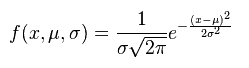
formula for normal distribution
  • e = constant (2.71828), the Poisson constant
  • x = control variable – (data being studied)
  • µ = population mean
  • σ = population standard deviation

Formulas for Population mean, Variance, and Standard Deviation.

Formula for Population Mean, Variance, Standard Deviation

N (capital N) refers to Population.

In this case, σ^2 is the variance.

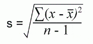
Formulas for Sample mean, Variance, and Standard Deviation.

Formula for Sample Mean, Variance, Standard Deviation
Formula for Sample Mean, Variance, and Standard Deviation

n (lowercase n) refers to sample size.

In this case, s^2 is the variance.

The population equations differ from the sample equations because we wish to reduce the “degrees of freedom” or increase our confidence in the sample.

Variation and Bell Shape

Adjusting to Center

You do not want to adjust an ongoing process to “center it.” This increases variation. The more you do this, the more the operator unduly influences the process, and the less the distribution will be shaped like a bell. See Quincunx demonstration.

Center of Process Variation

The peak of the normal curve indicates the average, which is the center of process variation.

5Ms & 1 P

When you have a bell-shaped curve, none of the 5 Ms or one P are unduly influencing the process.

Additional Notes:

Normal Distribution Videos

Good basic description of normal distribution

What is a standard normal distribution?

ASQ Six Sigma Black Belt Certification Normal Distribution Questions:

Question: For a normal distribution, two standard deviations on each side of the mean would include what percentage of the total population? (Taken from ASQ sample Black Belt exam.)

Answer:

Unlock Additional Members-only Content!

To unlock additional content, please upgrade now to a full membership.
Upgrade to a Full Membership
If you are a member, you can log in here.

ASQ Six Sigma Green Belt Certification Normal Distribution Questions:

Question: For a normal distribution, two standard deviations on each side of the mean would include what percentage of the total population?

(A) 95%
(B) 68%
(C) 47%
(D) 34%

Answer:

Unlock Additional Members-only Content!

To unlock additional content, please upgrade now to a full membership.
Upgrade to a Full Membership
If you are a member, you can log in here.

F-Distribution

What is the F-Distribution?

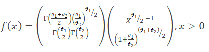
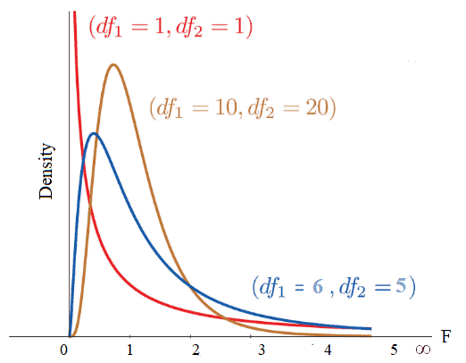
The F-distribution, also known as the Fisher-Snedecor distribution, is extensively used to test for equality of variances from two normal populations. F-distribution got its name after R.A. Fisher, who initially developed this concept in the 1920s. It is a probability distribution of an F-Statistic.

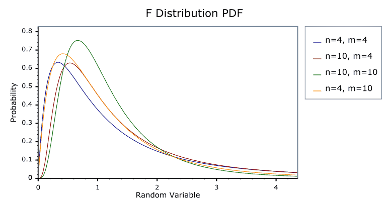
F-distribution probability density curve, positively skewed and bounded at zero on the left

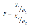
The F-distribution is generally skewed and also related to a Chi-Squared distribution. Additionally, the f-distribution is the ratio of the X1 random chi-square variable with degrees of freedom ϑ1 and the X2 random chi-square variable with degrees of freedom ϑ2. In other words, each Chi-Square random variable has been divided by its degrees of freedom.

Formula defining the F-distribution as the ratio of two chi-square random variables, each divided by its own degrees of freedom

The shape of the distribution depends on the degrees of freedom of numerator ϑ1 and denominator ϑ2.  

What are the properties of an F-distribution?

F-distribution curve labeled with its key properties: positively skewed, bounded at zero, and shape determined by numerator and denominator degrees of freedom
  • The F-distribution curve is positively skewed towards the right with a range from 0 to ∞.
  • The value of F is always positive or zero. No negative values.
  • The shape of the distribution depends on the degrees of freedom of numerator ϑ1 and denominator ϑ2.  
  • From the above graph, it is clear that the degree of skewness decreases with an increase in the degrees of freedom of the numerator and denominator.
  • The f-distribution curve can never be symmetrical; as the degrees of freedom increase, it becomes more nearly symmetrical.

When would you use the F-distribution?

The F-test compares more than one level of independent variable with multiple groups, which uses the F distribution. This is generally used in ANOVA calculations. When you compare the means of more than two groups, ANOVA’s F-test is the standard choice.

Example: In a manufacturing unit, torque values are key parameters in terminal squeeze welding. To check the significant effect of various torque (N·m) values of the squeeze welding, an operator set up trials of 5, 8, 10, and 12 N·m on terminals in four randomly selected batches of 30. ANOVA can determine whether the means of these four trials are different. ANOVA uses F-tests to statistically test the equality of means.

Assumptions of F-distribution

  • Assumes both populations are normally distributed.
  • Both populations are independent of each other.
  • When you compare two variances with an F test, the usual convention is to put the larger sample variance in the numerator so you only need the upper-tail table. (In ANOVA the ratio is always the between-groups mean square over the within-groups mean square.)

F-distribution Videos

Once you understand the F-distribution, see the F-Test page for how it’s actually used to compare variances, including the F-statistic calculation and worked examples for right-tailed, two-tailed, and left-tailed tests. For the full mathematical treatment and critical value tables, NIST’s Engineering Statistics Handbook is a reliable reference.

Worked Example: Calculating an F-Statistic

Two suppliers produce the same part. Supplier A’s output has a sample variance of 4.2; Supplier B’s has a sample variance of 1.8. To test whether A’s process is more variable (not just unlucky sampling), put the larger variance in the numerator: F = 4.2 / 1.8 = 2.33. Compare that F-statistic to the critical value from an F-table at your chosen alpha and the two samples’ degrees of freedom. If 2.33 exceeds the critical value, you have statistical grounds to say Supplier A’s process really is more variable, not just different by chance.

A Consistency Example

The F-ratio is a consistency comparison, and sports commentary makes this intuitive without any statistics vocabulary: “Team A is more consistent than Team B” is an informal F-test. If Team A scores between 2 and 4 runs almost every game and Team B swings wildly between 0 and 10, Team B has the larger variance. The F-distribution is just the formal, mathematical version of “how much more variable is one thing than another, and is that difference big enough to call real.”

F-Distribution in Practice: Before You Run a T-Test

One practical place the F-distribution shows up before you even get to ANOVA: deciding whether to run a pooled or unpooled (Welch’s) two-sample t-test. An F-test (or a simpler rule of thumb comparing standard deviations) checks whether the two groups’ variances are close enough to pool. If they’re not, using the pooled t-test formula anyway can throw off your results, which is why many statistical software packages run this variance check automatically before showing you the t-test output.

Frequently Asked Questions

Can an F-statistic be negative? No. Since it’s a ratio of two variances, and variances can never be negative, the F-statistic is always zero or positive.

What’s the difference between the F-distribution and the F-test? The F-distribution is the underlying probability distribution; the F-test is the hypothesis test that uses it to compare two variances (or, in ANOVA, to compare multiple group means at once by comparing variance between groups to variance within groups).

Why does the F-distribution need two separate degrees-of-freedom values? Because it’s a ratio of two independent chi-square variables, and each one has its own sample size behind it. The numerator degrees of freedom come from one group’s sample size, the denominator’s from the other’s, which is why an F-table has two axes instead of one.

What happens as both degrees of freedom get large? The F-distribution flattens out and becomes more symmetric, approaching a normal shape as sample sizes grow. With small samples it stays visibly right-skewed, which is part of why F-tests are sensitive to small sample sizes and why a reasonably sized sample matters for a reliable result.

Keep the ANOVA page and the F-Test page bookmarked alongside this one; together they cover the full path from “what is this distribution” to “how do I actually run the test” to “how do I use it to compare more than two groups at once.”

Process Control for Non-Normal Data

Process control for non-normal data involves monitoring and managing industrial or operational processes that produce non-normally distributed data. Non-normal data, also referred to as non-normally distributed data, are data points that do not follow a normal distribution or Gaussian distribution.

The objectives of process control remain the same as traditional process control: ensuring consistent product quality, minimizing defects, and maintaining stable production. However, when dealing with non-normal data, specific techniques and strategies are employed to effectively manage the process.

What is non-normal data?

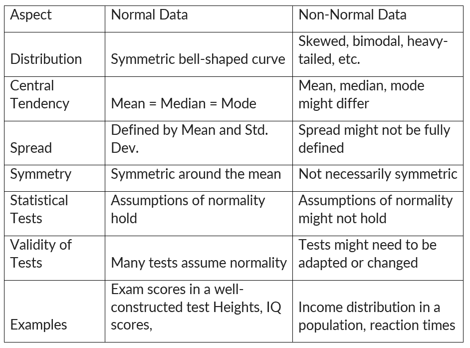
Non-normal data refers to data that deviates from a normal distribution. A normal distribution is a bell-shaped curve that is symmetrical around the mean. Non-normal data can be skewed (asymmetrical) or have outliers (extreme values).

When data doesn’t adhere to the characteristics of a normal distribution, it implies potential skewness or the presence of other distinct patterns. Such non-normal data can notably influence statistical analyses that presume a normal distribution, like t-tests or ANOVA (analysis of variance).

Process control for non-normal data
Normal vs. Non-Normal Data

How to identify non-normal data

Identifying non-normal data involves examining the distribution of data and looking for patterns that deviate from the characteristics of a normal distribution.

Visual Inspection:

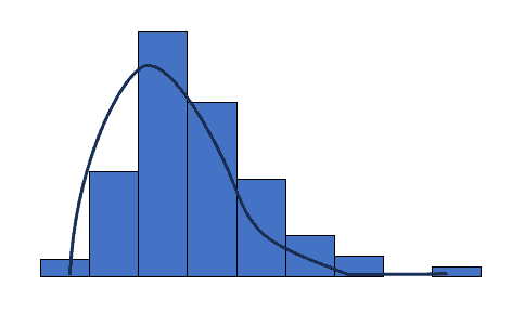
Histogram: Histogram is a bar chart showing the number of times an outcome is repeated. Create a histogram and observe its shape. Look for skewed distributions, multiple peaks, or irregular patterns.

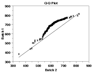
Q-Q Plot (Quantile-Quantile Plot): This plot compares the quantiles of data with the quantiles of a normal distribution. If the points deviate significantly from a straight line, the data might not be normal.

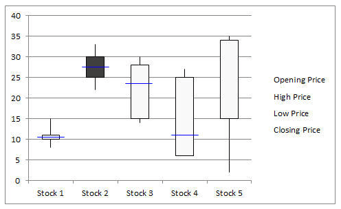
Box Plot: Box plots are used in statistics to graphically display various parameters at a glance. It helps to identify skewness and the presence of outliers.

Process Control for Non-Normal Data

Summary Statistics:

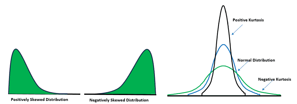
Skewness and Kurtosis: Calculate skewness and kurtosis values. Positive skewness and kurtosis values that deviate significantly from 0 and 3, respectively, can indicate non-normality.

Process Control for Non-Normal Data

Mean and Median: The median is the middle value when the data is arranged in ascending or descending order. If the mean and median significantly differ, it might suggest non-normality.

Process Control for Non-Normal Data

Statistical Tests:

Shapiro-Wilk Test: This test assesses the normality of data. If the p-value is below a certain threshold (e.g., 0.05), you might conclude that the data is not normally distributed.

Kolmogorov-Smirnov Test: Similar to the Shapiro-Wilk test, this test assesses the goodness of fit between the data and a normal distribution.

Process Control for Non-Normal Data

Sample Size:

With larger sample sizes, easy to detect deviations from normality that might not be noticeable with smaller samples. However, it’s important to consider the context and the practical significance of any deviations.

Why transform non-normal data into normal

Data transformation is a process of modifying the distribution of non-normal data to make it more closely resemble a normal distribution. This can be done using a variety of transformation techniques, such as the logarithmic transformation, the square root transformation, and the Box-Cox transformation.

Transformed data also tend to exhibit more symmetric distributions, rendering them more interpretable and facilitating clear communication of findings. Additionally, when comparing data across different groups or conditions, data transformation supports more meaningful and valid comparisons. However, it’s important to note that data transformation cannot guarantee the attainment of normal distribution. Also, the interpretation of transformed data can be less intuitive.

When to transform non-normal data to normal

  • For statistical tests or models that rely on the assumption of normality (e.g., t-tests, ANOVA, linear regression), and when the data significantly deviates from normality, data transformation can be employed to align with the assumption and enhance the validity of the results.
  • If the data contains extreme outliers that are influencing analyses, transformation can reduce their impact and help you focus on the underlying patterns in the data.
  • In the context of regression analysis, transforming the response variable (dependent variable) can help ensure that the residuals (the discrepancies between observed and predicted values) adhere to a normal distribution.
  • In cases where the variance of the data is not constant across groups or conditions (heteroscedasticity), transforming the data can help stabilize the variance, making statistical tests more reliable.
  • When the data is highly skewed (either positively or negatively), and this skewness is problematic for your analysis, transformation can make the data more symmetric.
  • For quality control settings, transforming data might be necessary to meet the assumptions of control charts or other quality control methods.

How to convert non-normal data to normal

  • Visual Assessment: Plot histograms, Q-Q plots, and other graphs to understand the initial distribution and identify the type of skewness.
  • Select Transformation: Based on the distribution characteristics, choose an appropriate transformation technique.
  • Apply Transformation: Apply the chosen transformation to the data. Be cautious with zero or negative values, as some transformations might not be suitable.
  • Assess Normality: After transformation, re-assess normality using the same techniques as before. Use statistical tests or visual comparisons.
  • Analysis: If the data is now closer to normality, then perform the desired analysis. If not, have to explore other transformation methods or consider using non-parametric methods.

Different transformation techniques

  • Logarithmic Transformation: Apply the natural logarithm (ln) to the data to approximate a normal distribution. This transformation is effective for positively skewed data and is particularly useful when dealing with data that span multiple orders of magnitude.
  • Box-Cox Transformation: The Box-Cox transformation encompasses a range of power transformations, including logarithmic, square root, and reciprocal transformations. By estimating a parameter (lambda) that maximizes normality, this method can be applied to data with both positive and negative skewness. The applicable formula is yl =yλ (λ is the power or parameter to transform the data). For instance, λ=2, the data is squared, and if λ=0.5, then a square root is required.
  • Square Root Transformation: Apply a square root transformation to the data to achieve normality. This method is suitable for data with moderate skewness, such as count data or data containing small positive values.
  • Reciprocal Transformation: Apply the reciprocal (1/x) to the data to transform it toward a normal distribution. This technique is beneficial for data that exhibits negative skewness, especially when dealing with data that includes large values.
  • Exponential Transformation: Utilize the exponential function (e^x) to improve the quality and normality of the data. The exponential transformation is advantageous for data with a left-skewed distribution, enhancing data usability.

Enacting Process Control with Non-normal Data

When dealing with non-normal data in process control, it’s essential to tailor the control strategies to the unique characteristics of the data distribution. Understand the specific features of the non-normal distribution, such as skewness or outliers.

Control charts, like the X-bar R chart, assume normality. However, for non-normal data, consider alternatives like individual control charts and median control charts that are explicitly designed for non-normal distributions. Additionally, data transformation can be an option if the data exhibits slight skewness or specific patterns.

Furthermore, when non-normal data consistently exceed the control limits, it’s essential to engage in process improvement efforts. Utilize structured frameworks like DMAIC (Define, Measure, Analyze, Improve, Control) to address root causes and enhance process stability. Also, continuously monitor and evaluate the control methods, adjusting the strategies as needed to ensure effective management of non-normal data for improved process stability and product quality.

Advantages of non-normal data

  • In real life, data often does not follow a perfect bell curve. Non-normal data is better at capturing the complex and diverse nature of real data.
  • Some statistical tests and methods are robust to deviations from normality. This means that they can still produce accurate results even when the data does not follow a normal distribution.
  • Non-normal data can reveal potential outliers or anomalies that might be hidden in normally distributed data.
  • Non-normal data can exhibit a wide variety of patterns, such as bimodal or multimodal distributions. This can help us to gain a richer understanding of the data.
  • The complexities of non-normal data may require the use of specialized statistical techniques. However, these techniques can ultimately lead to more accurate results.

Disadvantages of non-normal data

  • Many common statistical tests, like t-tests and ANOVA, assume a normal distribution for the data. Dealing with non-normal data can compromise the validity of these tests.
  • Using tests that assume normality on non-normal data can lead to wrong conclusions, such as false positives or false negatives.
  • The presence of non-normal data can make it more difficult to estimate parameters accurately.
  • Non-normal data, especially when it is skewed, can lead to inaccurate inferences about the population.
  • Applying statistical tests to non-normal data can reduce their effectiveness. This means that they may not be able to detect significant differences or relationships.
  • Interpreting statistical results derived from non-normal data can prove more challenging. This arises because the results may lack intuitiveness and tend to be more complex.
  • Data transformations can sometimes help to make non-normal data more normally distributed. However, this is not always possible.
  • Non-normal data is more susceptible to the influence of outliers. This means that outliers can have a greater impact on the results of statistical analyses.
  • Non-normal data may require the use of more complex modeling techniques in order to effectively capture the underlying patterns.

Important Videos

T Distributions & T Tests

What are T Distributions and T Tests?

Student’s t-distribution is used for finding confidence intervals for the population mean when the sample size is less than 30 and the population standard deviation is unknown. Further, Students’ t-test is divided into paired and unpaired t-tests. In other words, the t-distribution and t-tests are used to determine the likelihood of various conditions occurring for small sample sizes (<=30).

How Does the T Distribution Compare with the Z Distribution?

The z-distribution assumes a known standard deviation of the population, whereas the t-distribution is based on the sample standard deviation. The t-distribution is flatter and wider than the z-distribution.

The t-distribution becomes narrower (taller) as sample sizes increase and gradually becomes very close to the Normal Distribution. Both z and t-distributions are symmetric and bell-shaped, with a mean of zero.

Hypothesis Testing

A tailed hypothesis is an assumption about a population parameter. The assumption may or may not be true. The one-tailed hypothesis tests the hypothesis where the area of rejection is only in one direction. Whereas two-tailed, the area of rejection is in two directions. The selection of one or two-tailed tests depends upon the problem.

  • Null hypothesis- H0: The population means are the same; alternatively, the difference between the two population means is equal to the hypothesized difference (d). So, µ1 = µ2  orµ1– µ2 = d
  • Alternative hypothesis: µ1 ≠ µ2  orµ1– µ2 ≠ d (Two-tailed test)
  • µ1 < µ2  orµ1– µ2 < d (left-tailed)
  • µ1 > µ2  orµ1– µ2 > d (Right-tailed)

What is T-score?

A t-score is the number of standard deviations from the mean in a t-distribution. You can typically look up a t-score from the t-table.

T-scores are primarily used to find:

  • Upper and lower bounds of a confidence interval of normally distributed data.
  • The p-value of the test statistic.

What is the T Distribution Table?

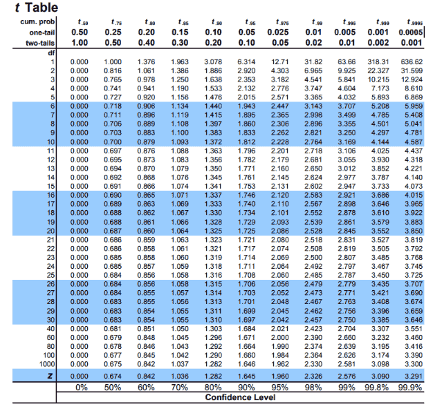
The t-distribution table values are critical values of the t-distribution. The column header is the t-distribution probabilities (alpha). The row names are the degrees of freedom (df). Student t-table gives the probability that the absolute t value with a given degrees of freedom lies above the tabulated value.

http://www.sthda.com/english/wiki/t-distribution-table
  • The degrees of freedom of the t-test
  • The number of tails of the t-test (one-tailed or two-tailed)
  • The alpha level of the t-test (common choices are 0.01, 0.05, and 0.10)

When Would You Use a T Distribution or a T Distribution Table?

T-distributions are most likely used to compare two process means. It is a hypothesis test of means.

You would use these in the following specific hypothesis tests:

  • One-Sample T-Test: The One Sample T-Hypothesis Test (Student’s T-Test) allows for comparing the (small) population mean to some hypothesized value or one sample mean to determine if they are significantly different.
  • Two-Sample T-Test: A two-sample t-hypothesis test, also known as an independent t-test is used to analyze the difference between two unknown population means. The two-sample t-test is used when the two small samples (n< 30) are taken from two different populations and compared. The underlying chart makes use of the T distribution.
  • Paired T-Test: A paired t-test (Paired T-Distribution, Paired T-Test, Paired Comparison test, Paired Sample Test) is a statistical method to test whether the average difference between the two measurements is statistically significant from zero.

Student’s T Distribution Example Questions

We can use Student’s t-distribution to find confidence intervals for the population mean when the sample size is less than 30, and the population standard deviation is unknown.

Confidence of a mean 1

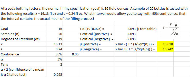
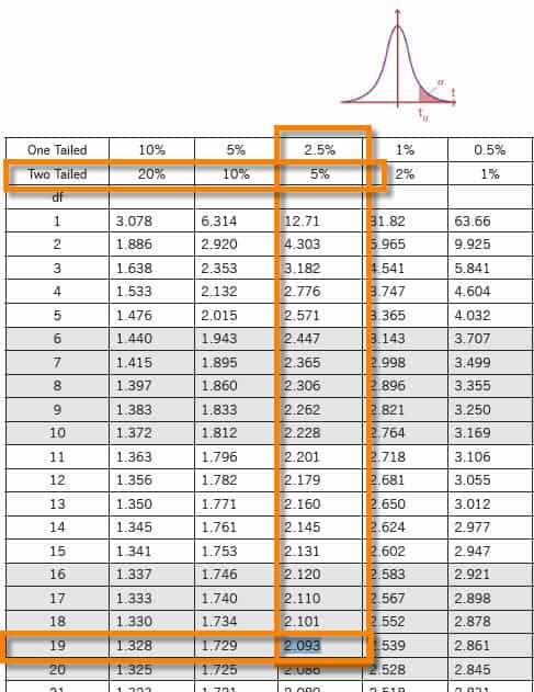
At a soda bottling factory, the normal filling specification (goal) is 16 fluid ounces. A sample of 20 bottles is tested with the following results: x = 16.13 fl oz and s = 0.24 fl oz. What interval would allow you to say, with 95% confidence, that the interval contains the actual mean of the filling process?

Student 1 and T Distribution & T Tests
Student 1 chart

Confidence of a mean 2

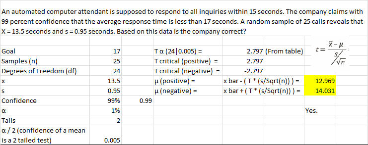
An automated computer attendant must respond to all inquiries within 15 seconds. The company claims with 99 percent confidence that the average response time is less than 17 seconds. A random sample of 25 calls reveals that X = 13.5 seconds and s = 0.95 seconds. Based on this data, is the company correct?

Student 2 chart and T Distribution & T Tests
Student 2

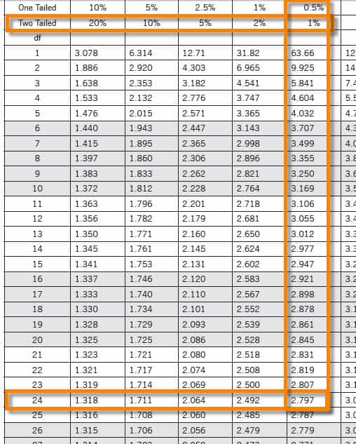
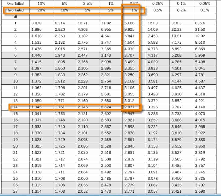
Confidence of a mean 3

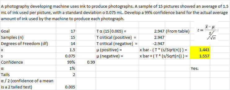
A photography-developing machine uses ink to produce photographs. A sample of 15 pictures showed an average of 1.5 mL of ink used per picture, with a standard deviation o 0.075 mL. Develop a 99% confidence band for the actual average amount of ink the machine uses to produce each photograph.

Student 3 chart
Student 3

Confidence Interval Question Using T-Score

Question: A factory produces tennis balls. Quality control takes a sample of 19 balls from one day’s production in the factory. The mean weight of the sample balls is 58.2g. The standard deviation for the sample balls is 0.4g. Calculate the confidence interval with a confidence level of 95%.

Calculation: The sample size is too small to use a Z-score. Instead, use a T-score, which uses a t-distribution. Finding a confidence interval for a mean is a two-tailed test.

You’ll need an alpha score. To calculate it, use this simple equation:

α = (100% – confidence level%)= (100% – 95%) = 5%

You also need the degrees of freedom (df), which is the number of samples minus one. Or in equation form:

df = n – 1

df for this question is 18.

So, use a T-table to look up the T-score needed for a two-tailed test with an α of 5% and a df of 18: the answer is 2.101.

tα/2=2.101, X̅=58.2, σ=0.4 and n=19

Margin of error E =tα/2*σ/√n = 2.101*0.4/√19 = 0.192

Confidence interval = X̅±tα/2*σ/√n = 58.2±0.192

Answer: Hence, a 95% confidence interval for tennis balls produced in the factory is 58.008 to 58.392g.