Chi-Square Goodness of Fit Test

A chi-square goodness-of-fit (GOF) test checks how well an observed categorical data distribution fits an expected distribution. In other words, it tests whether the frequencies observed in different categories match some hypothesized frequencies. This is useful when you have one categorical variable and a theory or historical data about what the distribution of that variable should be. For example, you might want to verify if defect occurrences follow a Poisson distribution, or if customer preferences are evenly distributed among choices. The chi-square GOF test is a non-parametric test (no assumption of normality; it deals directly with category counts).

When to use Chi-Square Goodness of Fit?

A chi square goodness-of-fit test can be conducted when there is one categorical variable with more than two levels. If there are exactly two categories, then a one proportion z test may be conducted.

Reference.

The chi-square goodness-of-fit test requires 2 assumptions^2,3:

1. Independent observations;

2. For 2 categories, each expected frequency EiEi must be at least 5.

For 3+ categories, each EiEi must be at least 1 and no more than 20% of all EiEi may be smaller than 5.

Reference

When to use: Use a GOF test in Six Sigma during Measure or Analyze when you need to validate distributional assumptions. For instance, if you assume defects per hour follow a Poisson distribution, a GOF test can confirm or refute that. Or if historical data suggest a certain proportional breakdown of defect causes, you can test if current data still fits that pattern. This helps ensure you’re using the correct statistical models and can reveal changes in process behavior.

Hypotheses: Typically, for a goodness-of-fit test:

• H₀ (null hypothesis): The observed distribution fits the expected distribution. (No significant difference between observed and expected frequencies.)
• H₁ (alternative hypothesis): The observed distribution does not fit the expected distribution (at least one category’s frequency is significantly different from expected).

In plain terms, H₀ assumes any differences between observed and expected counts are just due to random chance, while H₁ asserts that the differences are too large to be random – indicating the distribution has changed or the assumption was wrong.

Assumptions: Each observation falls into one of the categories, and you have a sufficiently large sample such that expected counts in each category aren’t too low. A common rule of thumb is that expected counts should be at least 5 in each category (or if that’s not possible, no more than 20% of categories have expected < 5)sixsigmastudyguide.com. If expected frequencies are very small, the chi-square approximation may not be accurate (you might need to combine categories or use an exact test).

Steps to Perform a Chi-Square Goodness-of-Fit Test

1. Define the hypotheses:
   • Null (H₀): The observed category proportions are equal to the expected proportions (no difference between observed and expected distribution).
   • Alternative (H₁): The observed proportions differ from the expected (at least one category is not in line with the expected distribution).
2. Choose a significance level (α): Commonly α = 0.05 (5% significance) is used, corresponding to 95% confidence.
3. Collect data and calculate expected frequencies: Determine the expected count for each category under H₀. Often this is done by multiplying the total sample size by the expected percentage for each category. Expected values might be given by a theoretical distribution (e.g., a probability model or historical proportions). Ensure the total of expected counts equals the total observations.
4. Compute the chi-square statistic:
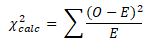
   χ2=∑i=1k(Oi−Ei)2Ei,\displaystyle \chi^2 = \sum_{i=1}^{k} \frac{(O_i – E_i)^2}{E_i},χ2=i=1∑k​Ei​(Oi​−Ei​)2​,
   where O_i is the observed frequency for category i and E_i is the expected frequencysixsigmastudyguide.comsixsigmastudyguide.com. Each term $(O – E)^2/E$ measures the squared difference relative to expectation. Sum these across all k categories to get χ².
5. Determine degrees of freedom: For goodness-of-fit, df = (number of categories – 1) minus any parameters estimated from the data. If the expected proportions are completely specified in advance, df = k – 1. (For example, if you have 4 categories, df = 3.) If you estimated parameters (like the mean of a Poisson from the data), subtract those as well.
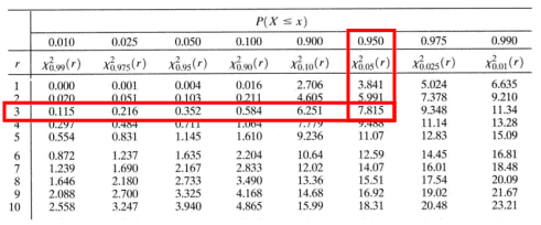
6. Find the critical value: Because this test is right-tailed (we care about large χ²), find the critical χ² value for the chosen α and the calculated degrees of freedom. This value comes from the chi-square distribution table. For instance, at α = 0.05 and df = 3, the critical value is 7.815 (meaning that 5% of the time, a random χ²(3) would exceed 7.815). If using p-value approach, compute p (the area to the right of your χ² statistic).
7. Make a conclusion: Compare your χ² statistic to the critical value. If χ²_stat > χ²_critical (or p-value < α), reject H₀. This means the differences between observed and expected are statistically significant – the data do not fit the expected distribution. If χ²_stat is smaller than critical (p > α), you fail to reject H₀, meaning any differences are small enough to be explained by chance, and the distribution fits as assumed.

Goodness-of-Fit Example: Did Our Customer Distribution Change?

To illustrate, consider a realistic Six Sigma scenario: A loyalty program manager wants to know if the age distribution of the company’s priority customers has changed over the last decade. Ten years ago, the company categorized its priority customers by age and found the distribution to be: 15% were under 25, 40% were 25-40 years old, 25% were 40-60, and 20% were over 60. Now, in the Analyze phase of a project, the manager takes a random sample of 500 current priority customers and observes their age breakdown. We can use a chi-square goodness-of-fit test to see if the current sample’s distribution differs from the 2010 baseline.

Expected age distribution of priority customers in 2010 (historical baseline). Each percentage represents the proportion of customers in that age group (SixSigmaStudyGuide.com).

From the 2010 data (expected distribution):

• Under 25: 15%
• 25–40: 40%
• 40–60: 25%
• Over 60: 20%

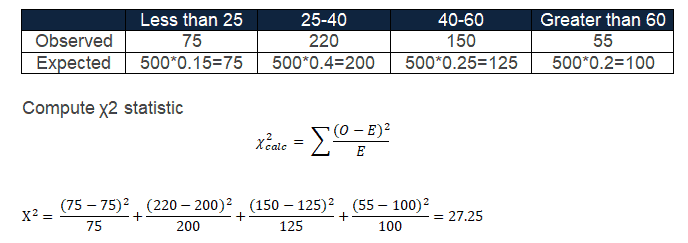
If we expect those proportions to still hold, the expected frequencies out of 500 customers would be:
Under 25: 0.15 * 500 = 75
25–40: 0.40 * 500 = 200
40–60: 0.25 * 500 = 125
Over 60: 0.20 * 500 = 100

Observed age distribution of a 2020 sample of 500 priority customers (SixSigmaStudyGuide.com). These are the actual counts in each age group from the sample.

The observed frequencies in the 2020 sample of 500 are:
Under 25: 75
25–40: 220
40–60: 150
Over 60: 55

Let’s run the chi-square GOF test at 95% confidence (α = 0.05). First, state hypotheses:

• H₀: The 2020 age distribution matches the 2010 distribution (no change).
• H₁: The 2020 age distribution differs from 2010 (at least one age group has a different proportion).

We already have expected (E) and observed (O) counts. Now calculate the χ² statistic:

• Under 25: O=75, E=75 ⇒ (75–75)²/75 = 0
• 25–40: O=220, E=200 ⇒ (220–200)²/200 = (20)²/200 = 400/200 = 2.0
• 40–60: O=150, E=125 ⇒ (150–125)²/125 = 625/125 = 5.0
• Over 60: O=55, E=100 ⇒ (55–100)²/100 = (–45)²/100 = 2025/100 = 20.25

χ²_stat = 0 + 2.0 + 5.0 + 20.25 = 27.25 (approximately).

Degrees of freedom = 4 categories – 1 = 3. For df = 3 at α = 0.05, the chi-square critical value is 7.815sixsigmastudyguide.com. Our test statistic (27.25) is much larger than 7.815, falling deep in the right tail beyond the cutoff. This means the probability of seeing a χ² that large under H₀ is extremely low. We therefore reject H₀.

Conclusion: The sample data provide strong evidence that the age distribution of priority customers in 2020 is different from the 2010 distribution. Specifically, the chi-square contributions suggest the biggest differences are in the older age groups (the “Over 60” category had far fewer people than expected, contributing heavily to χ²). In Six Sigma terms, if this was a KPI or a customer demographic critical to quality, we’d note that the customer base has shifted significantly over the decadesixsigmastudyguide.com.

(Notice that this GOF test was one-tailed (right-tail) because only a large χ² (indicating a big deviation) would lead us to reject H₀. Small deviations wouldn’t).

Chi square goodness of fit test specifically tells how well a categorical (nominal or ordinal) sample distribution fit into a hypothetical distribution. In other words, it is the test used to check if the sample data is consistent with a hypothesized distribution of the population. The goodness of fit test is used to determine the observed sample distribution matches or fits the expected values; hence we use the term goodness of fit.

The goodness of fit is a non-parametric test because it does not rely on estimates of a population parameter like mean or variance to make an inference on the characteristics of the population.

Structure of a Chi-Square Goodness of Fit Test

The goodness of fit tests is structured in cells; therefore, the observed frequency goes in each cell. Furthermore, the distribution you are trying to match would have a theoretical frequency. Then, the chi-square is summed across all cells.

Use the data values structured into cells, explicitly requiring a calculated chi-square test statistic. The unknown distribution is tested; likewise, the Degrees of Freedom vary according to the distribution.

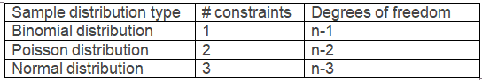
GOF Distribution  | Degrees of Freedom

Normal | # cells – 3

Poisson | # cells – 2

Binomial | # cells – 2

Uniform | # cells – 1

Steps to perform Chi-Square goodness of fit

Step1:

Firstly, define the null hypothesis and alternative hypothesis

• Null hypothesis (H₀): There is no difference between the observed value and the expected value
• Alternative hypothesis (H₁): There  is a significant difference between the observed value and the expected value

Step 2:

Secondly, specify the level of significance.

Step 3:

Thirdly, compute the χ2 statistic.

• O is the observed value
• E is the expected value

Step 4:

Fourthly, calculate the degree of freedom:

The degrees of freedom in chi-square test depends on the sample distribution

Step 5:

Then, find the critical value based on degrees of freedom.

Step 6:

Finally, draw the statistical conclusion:

If the test statistic value is greater than the critical value, reject the null hypothesis. Hence, we can conclude that there is a significant difference between the observed value and the expected value.

Chi-Square goodness of fit test Example 1: Did the Distribution Change?

Ten years ago, US airlines categorized the priority customers (those who completed 10,000 miles traveled in a year) based specifically on age:

Similarly, in 2020, 500 priority passengers were sampled, and below are the results:

At a 95% confidence level, would you conclude that the population distribution of priority customers changed in the last 10 years?

• Null hypothesis (H₀): The sample data meet the expected distribution.
• Alternative hypothesis (H₁): The sample data does not meet the expected distribution.

Level of significance: α=0.05:

Degrees of freedom = number of categories (n)= 4

n-1 =3

Chi-square critical value for 3 degrees of freedom =7.815

The test statistic value is greater than the critical value; hence, we can reject the null hypothesis.

So, we can conclude that the priority customers in 2020 are different than those expected based on the 2010 population.

Download Chi-Square Goodness of Fit Exemplar

Chi-Square Normality Test

Many statistical techniques (regression, ANOVA, t-tests, etc.) rely on the assumption that data is normally distributed. Hence, the chi-square goodness of fit test is one of the good options to check whether the data follows a normal distribution.

Furthermore, the chi-square goodness of fit test is an alternative to the Anderson-Darling test, Kolmogorov-Smirnov (K-S) test, and Shapiro-Wilk test to test the normality.

Similar to other statistical hypothesis tests, the chi-square goodness of fit test also needs to compute the test statistics and find the critical value for a given degree of freedom and confidence level. If the chi-square value is greater than the critical value, reject the null hypothesis.

How to conduct Chi-Square goodness fit normality test

• Determine the null hypothesis, i.e. data is sampled from a normal distribution and alternative hypothesis.
• Compute the sample mean as well as the standard deviation.
• Then, define the confidence level.
• Bin the data: Determine non-overlapping bins, and then count values in each bin
• Furthermore, find the cumulative probability for each category endpoint.
• After that, compute the probability that a randomly selected value would go into each category.
• Find expected observations for each bin, which is the product of the probability of observation would fall in the bin compared to the sample size (n).
• Likewise, compute the chi-square statistic. χ2 = Σ [ ( Observed frequency – Exp frequency) 2 / Exp frequency].
• Find the degrees of freedom based specifically on the number of categories or bins. The degrees of freedom for the chi-square goodness of fit test is always the number of categories-1-2(two estimated parameters, mean and standard deviation) = k-3 (note: valid if mean and standard deviation is not given).
• Find the critical value based on degrees of freedom.
• Finally, draw the statistical conclusion: If the test statistic value is greater than the critical value, reject the null hypothesis.

Chi-Square normality test example

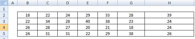
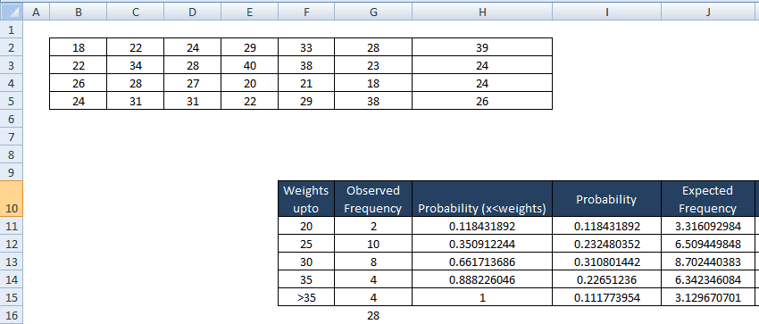
Example: 28 students’ weights (in kgs) are collected in ABC school. Test whether the data is normally distributed, given that the confidence level is 95%.

• H₀: Students’ weights in an ABC school follow a normal distribution
• H₁: Students’ weights in an ABC school do not follow a normal distribution

Firstly, compute the sample mean and standard deviation.

• Select all the data and enter” =Average(B2:H5)” for mean and “ Stdev(B2:H5)” for standard deviation
• Confidence level = 95%

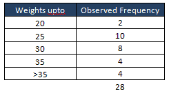
Secondly, bin or categories the data and count the values

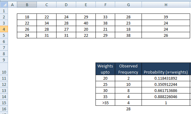
Thirdly, find the cumulative probability for each category endpoint.

• In cell H11 type NORMDIST (20, L2, L4, TRUE),
• Similarly H12 =  NORMDIST (25, L2, L4, TRUE),
• H13 =  NORMDIST (30, L2, L4, TRUE),
• H14=  NORMDIST (35, L2, L4, TRUE),
• H15 =  NORMDIST (∞, L2, L4, TRUE),

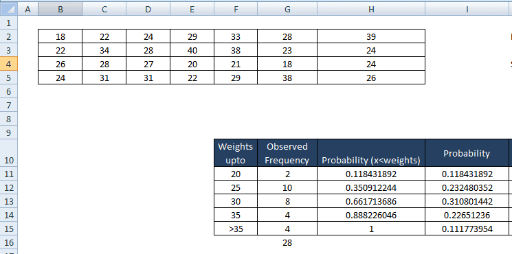
Fourthly, compute the probability that a randomly selected value would go in each category.

• For I 11 cell, ie less than 20 copy the same value ie 0.118431892
• In cell I 12, i.e. values between 25 to 20= H12-H11 = 0.350912244-0.118431892 = 0.232480352
• Similarly for I13 = H13-H12=0.310801442
• I14 = H14-H13 = 0.226512236
• I15 = H15-H14 = 0.111773954

Then, find expected observations in each bin, which is the product of the probability of observation would fall in the bin to the sample size (n) =28.

• J11 = I11*$G$16 = 3.316092984
• Similarly, J12=I12*$G$16=6.509449848
• J13=I13*$G$16=8.702440383
• J14=I14*$G$16=6.342346084
• J15= I15*$G$16=3.129670701

Finally, find the chi-square statistic. χ² = Σ [ ( Observed frequency – Exp frequency) ² / Exp frequency]

• K11 = (G11-J11)²/J11 = 0.522331777
• Similarly, K12 =  (G12 – J12)² / J12 = 1.871731198
• K13=(G13-J13)²/J13=0.056699325
• K14=(G14-J14)²/J14 = 0.865071869
• K15=(G15-J15)²/J15 = 0.242029645
• Then, find the sum of chi-square values = K16= sum(K11:K15) =3.55786

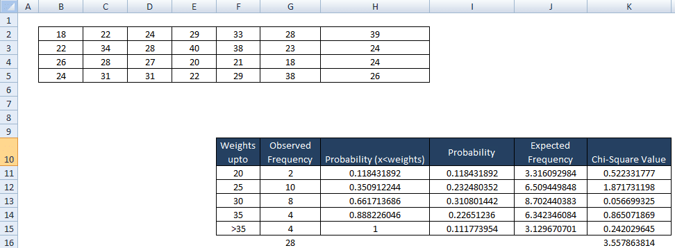
• Following that logic, the Degrees of freedom = No of categories -3 =5-3 =2
• Consequently, the Critical value =5.991

Conclusion: The chi-square value of 3.557 is less than the critical value of 5.991. In hypothesis testing, a critical value is a point on the test distribution that is compared to the test statistic to determine whether to reject the null hypothesis. If the chi-square calculated was smaller than the critical value, then the data did fit the model, therefore, failed to reject the null hypothesis. So, students’ weights in ABC school follow a normal distribution.

Download Chi-Square Test of Normality Exemplar

Chi-Square Normality Testing

• https://www.statisticshowto.datasciencecentral.com/chi-square-test-normality/