Chi Square Distribution & Hypothesis Test

The Chi-Square (χ²) distribution is a continuous probability distribution that plays a vital role in Six Sigma statistical analysis and hypothesis testing. It describes the distribution of a sum of squared random variables (usually z-scores). This distribution is always non-negative (since squares are always positive) and is typically right-skewed, especially for lower degrees of freedom.

The Chi-Square (χ2) distribution is the best method to test a population variance against a known or assumed value of the population. A Chi-Square distribution is a continuous distribution with degrees of freedom. As the degrees of freedom increase, the chi-square curve becomes more symmetric and approaches a normal distribution. Six Sigma practitioners (Green Belts and Black Belts) encounter the chi-square distribution when they need to analyze variability or test hypotheses about categorical data during a DMAIC project.

The best part of a Chi-Square distribution is that it describes the distribution of a sum of squared random variables. It is also used to test the goodness of fit of data distribution, whether a data series is independent, and for judging the confidences surrounding variance and standard deviation for a random variable from a normal distribution.

This guide will explain what the chi-square distribution is, why it’s important in Six Sigma, how to conduct various chi-square hypothesis tests, and when to use each test in the DMAIC process.

What Is the Chi-Square Distribution?

The chi-square distribution is a family of distributions defined by a parameter called degrees of freedom (df). Intuitively, you can think of degrees of freedom as related to sample size – for example, if you sum the squares of k independent standard normal variables, the result follows a χ² distribution with k degrees of freedom. Key properties of the chi-square distribution include:

• Non-negativity: χ² values range from 0 to ∞ (no negative values, since it’s a sum of squares).
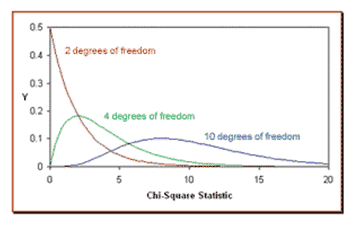
• Shape depends on degrees of freedom: With low df, the distribution is highly skewed right (a long tail to the right). As df increases, the distribution becomes more bell-shaped and approaches symmetry.
• Mean and variance: The mean of a χ² distribution is equal to its degrees of freedom, and the variance is twice the degrees of freedom. For example, a χ² with df = 6 has mean 6 and variance 12.
• Relation to normal distribution: A chi-square distribution with a large df (say df ≥ 30) is approximately normal. In fact, when df increases, the χ² probability density function begins to look symmetric like the normal curvesixsigmastudyguide.com.

These properties mean that small χ² values cluster near zero, and large values are rarer (in the right tail). This characteristic is exactly what makes the chi-square distribution useful for hypothesis testing – we use it to quantify how far our observed data deviate from expectation.

In practice, chi-square statistics often measure the discrepancy between observed data and what we expect under some hypothesis. If the chi-square statistic is small, it suggests the observed data are close to what was expected. If it’s large, it means there’s a big gap between observation and expectation – so large χ² values often indicate that the observed pattern is unlikely to be due to random chance under the null hypothesis.

Why Is Chi-Square Important in Six Sigma?

Six Sigma projects focus on reducing defects and variability. While many Six Sigma analyses involve means and the normal distribution, practitioners also need to understand variability and categorical data relationships. The chi-square distribution is central to several hypothesis tests that Six Sigma teams use to analyze variation and categorical factors in the Analyze phase (and sometimes in Measure/Improve phases). Usually, the goal of the Six Sigma team is to find the level of variation of the output, not just the mean. Chi-square tests help in this pursuit by enabling you to:

• Evaluate process variance: The chi-square is the distribution used to test a population variance or standard deviation against a target or baseline. For example, you might verify in the Measure phase that a process’s variance is within an acceptable range, or in the Improve phase that an improvement initiative significantly reduced variability. (This is done via the chi-square test for a single variance, described later.)
• Assess distribution fit: Six Sigma often assumes normality for process metrics, but what if the data are not normal? A chi-square goodness-of-fit test can check if your data follow a particular distribution (e.g., normal, Poisson, etc.). This could occur in Measure/Analyze when you need to validate distribution assumptions for capability analysis or determine if a count of defects fits a Poisson model.
• Test for independence (association): In Analyze, you may need to determine whether two categorical factors are related. For example, are defect types independent of the machine or shift? A chi-square test of independence can reveal whether there is a statistically significant association between two categorical variables (e.g., factor and defect occurrence), which helps pinpoint root causes. If the test shows dependence, you’ve found a clue on where to focus improvements.
• Analyze frequency counts and proportions: Chi-square tests handle data in frequency form (counts in categories). This is common in survey data or whenever outcomes are classified into categories. For instance, a Six Sigma team might survey customers about preferences (categorical responses) or classify defect reasons into categories – chi-square analysis can determine if those frequencies differ from expectations or differ across groups.

In summary, the chi-square distribution underpins tools for variation analysis and categorical data analysis in Six Sigma. It is especially relevant during Analyze (hypothesis testing for root cause analysis) but also appears in Measure (for baseline distribution checks or variance tests) and Improve (to confirm changes in variation). Knowing when and how to use chi-square tests during DMAIC ensures you select the right tool for questions about variability or categorical factors.

History of Chi-Square

Karl Pearson (1857 – 1936), the father of modern statistics (founded the first statistics department in the world at University College London), came up with the Chi-Square distribution. Pearson’s work in statistics began when he developed a mathematical method for studying the process of heredity and evolution. Later, the Chi-Square distribution came about as Pearson tried to find a measure of the goodness of fit of other distributions to random variables in his heredity model.

Chi-Square Statistic

A Chi-Square distribution may skew to the right or with a long tail toward the significant values of the distribution. The overall shape of the distribution will depend on the number of degrees of freedom in a given problem. The degree of freedom is one less than the sample size.

Chi-Square Properties

• The mean of the distribution is equal to the number of degrees of freedom: μ=ϑ.
• The variance equals two times the number of degrees of freedom: σ2 = 2*ϑ.
• When the degrees of freedom are greater than or equal to 2, the maximum value for Y occurs when χ2=ϑ-2.
• As the degrees of freedom increase, the Chi-Square curve nears a normal distribution.
• As the degrees of freedom increase, the symmetry of the graph also increases.
• Finally, It may be skewed to the right, and since the random variable it is based on is squared, it has no negative values. As the degrees of freedom increase, the probability density function begins to appear symmetrical.

The formula for the probability density function of the Chi-Square distribution is

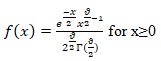
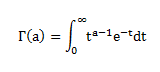
Where ϑ is the shape parameter, and Γ is the gamma function.

The formula for the gamma function is

Chi-Square (χ²) Hypothesis Test

Usually, the goal of the Six Sigma team is to find the level of variation of the output, not just the mean of the population. Above all, the team would like to know how much variation the production process shows about the target to see what changes are needed to reach a process free of defects.

For a comparison between several sample variances or a comparison between frequency proportions, the standard test statistic called the Chi-Square χ2 test will be used. So, the distribution of the Chi-Square statistic is called the Chi-Square distribution.

Types of Chi-Square Hypothesis Tests

The Chi-Square test is best suited for:

Case I: Testing whether a sample’s variance matches a known population variance (Chi-Square test for a single variance).

Case II: Testing whether observed frequencies differ significantly from expected frequencies, as in tests of independence or goodness-of-fit with categorical data.

I’ll give an overview of each below and link to pages where you can find more information on exactly how to perform both.

A hypothesis test is used to assess claims about a population parameter. Whether the test is one-tailed or two-tailed depends on the direction of the alternative hypothesis.

• A one-tailed test checks whether a parameter is significantly greater than or less than a certain value (rejection area in one tail).
• A two-tailed test checks whether a parameter is simply different from the hypothesized value (rejection areas in both tails).

The Chi-square test is commonly used for:

• Goodness-of-fit tests
• Tests of independence
• Tests for a single population variance

Key characteristics of the Chi-square distribution:

• It is non-negative (values ≥ 0)
• It is not symmetric — it is right-skewed
• The shape depends on the degrees of freedom (df)
• For a variance test: df=n−1df = n – 1df=n−1

⚠️ Important distinction:

When testing frequency data (e.g., for independence or goodness-of-fit), you do not need the population variance.

When testing a single variance, you must know the population variance to form your null hypothesis.

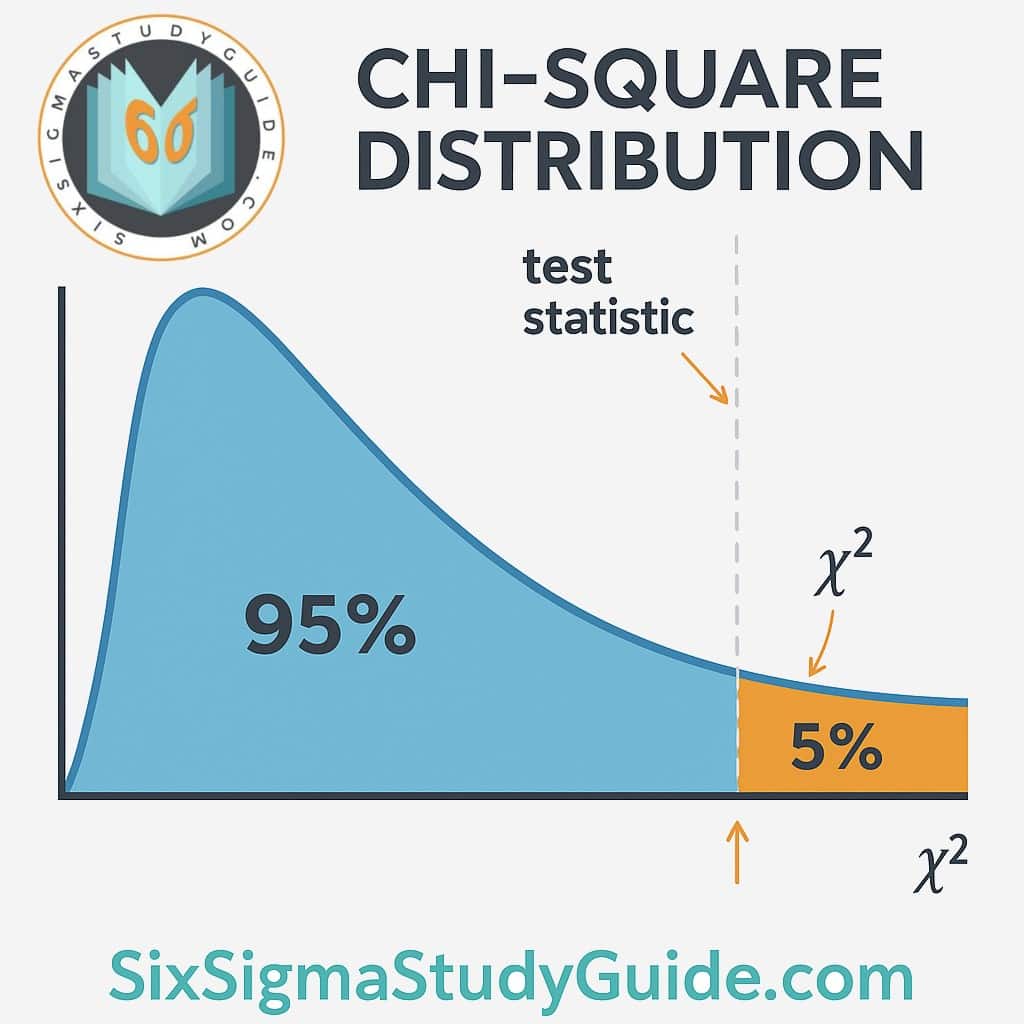
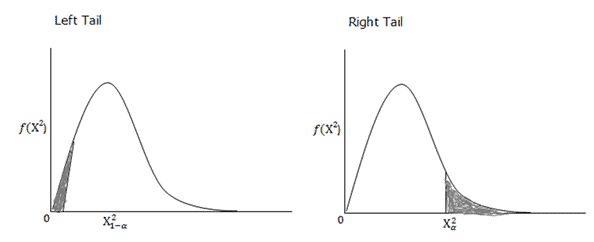
Left tail and Right tailed χ² distribution:

Right-Tailed vs. Left-Tailed vs. Two-Tailed Chi-Square Tests

Most chi-square hypothesis tests are naturally one-tailed, but it’s important to understand which tail (right or left) is being used. The chi-square distribution is not symmetric, and it’s typically right-skewed, so the “tail” refers to the upper end (right tail) or lower end (left tail) of the distribution curve.

Left-tailed vs. right-tailed regions in a χ² distribution (SixSigmaStudyGuide.com). In a right-tailed test, large χ² values (far right) indicate significance. In a left-tailed test, very small χ² values (far left) indicate significance.

• Right-Tailed Tests: By far the most common case. Goodness-of-fit and independence tests are almost always right-tailed. Why? Because the test statistic in these cases is χ² = Σ (O−E)²/E, which is always positive. The greater the discrepancy between Observed (O) and Expected (E) frequencies, the larger χ² becomes, pushing it into the right tail of the distribution. If the χ² value is extremely large (beyond a critical value in the right tail), it indicates the observed frequencies deviate significantly from expectations, and we reject the null hypothesissixsigmastudyguide.comsixsigmastudyguide.com. In other words, these tests only have one rejection region on the high side of the χ² curve.
• Left-Tailed Tests: These are rare for chi-square, but they occur in specific scenarios – particularly the chi-square test for a single variance when you want to see if a variance is significantly smaller than a target value. In a left-tailed χ² test, the rejection region is in the left tail (low values) of the distribution. A small χ² statistic would indicate observed variance is much lower than expected. For example, if you hypothesize that a new process’s variance is less than the old variance, you’d use a left-tailed test (lower variance yields a smaller χ² value). If the test statistic falls below a critical value near the left tail, you reject the null and conclude the variance is significantly lower. (We’ll see an example with queue wait times shortly.)
• Two-Tailed Tests: There is no built-in two-tailed version of the chi-square in the way we have for Z or t (because χ² ≥ 0 only). However, you can conduct a two-tailed test on variance by splitting α into both tails of the χ² distribution. This is used if you want to detect any significant difference (either increase or decrease) in variance. In practice, a two-tailed chi-square test for variance means you have two critical values: one in the right tail and one in the left tail. You would reject the null hypothesis if the χ² statistic is either too high (above the upper critical value) or too low (below the lower critical value). Two-tailed chi-square tests are less common in Six Sigma because usually one is checking either for an increase or a decrease in variation, not just any change. But it’s conceptually similar to two-tailed tests elsewhere – you’re defining an extreme region on both ends of the distribution.

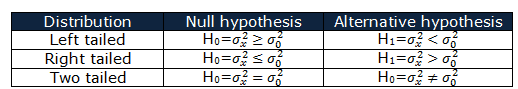
Selecting the Correct Tail: A common mistake is confusing which tail to use. Remember that for goodness-of-fit and independence tests, you always use the right tailsixsigmastudyguide.com – a large χ² is the signal that the observed data don’t match the null hypothesis expectation. For variance tests, it depends on your alternative hypothesis:

• H₁: σ² > σ₀² (looking for greater variability) – use a right-tailed test.
• H₁: σ² < σ₀² (looking for reduced variability) – use a left-tailed test.
• H₁: σ² ≠ σ₀² (any difference) – use a two-tailed approach (both tails).

In the sections below, we’ll highlight the tail for each type of test. We’ll also discuss how to find the correct critical values from a chi-square table for each case in a later section.

Chi-Square Goodness-of-Fit Test

A chi-square goodness-of-fit (GOF) test checks how well an observed categorical data distribution fits an expected distribution. In other words, it tests whether the frequencies observed in different categories match some hypothesized frequencies. This is useful when you have one categorical variable and a theory or historical data about what the distribution of that variable should be. For example, you might want to verify if defect occurrences follow a Poisson distribution, or if customer preferences are evenly distributed among choices. The chi-square GOF test is a non-parametric test (no assumption of normality; it deals directly with category counts)sixsigmastudyguide.com.

When to use: Use a GOF test in Six Sigma during Measure or Analyze when you need to validate distributional assumptions. For instance, if you assume defects per hour follow a Poisson distribution, a GOF test can confirm or refute that. Or if historical data suggest a certain proportional breakdown of defect causes, you can test if current data still fits that pattern. This helps ensure you’re using the correct statistical models and can reveal changes in process behavior.

Hypotheses: Typically, for a goodness-of-fit test:

• H₀ (null hypothesis): The observed distribution fits the expected distribution. (No significant difference between observed and expected frequencies.)
• H₁ (alternative hypothesis): The observed distribution does not fit the expected distribution (at least one category’s frequency is significantly different from expected).

In plain terms, H₀ assumes any differences between observed and expected counts are just due to random chance, while H₁ asserts that the differences are too large to be random – indicating the distribution has changed or the assumption was wrong.

Assumptions: Each observation falls into one of the categories, and you have a sufficiently large sample such that expected counts in each category aren’t too low. A common rule of thumb is that expected counts should be at least 5 in each category (or if that’s not possible, no more than 20% of categories have expected < 5)sixsigmastudyguide.com. If expected frequencies are very small, the chi-square approximation may not be accurate (you might need to combine categories or use an exact test).

Learn more about Chi-Square Goodness of Fit Test including how to create one, a step by step walkthrough, and specifi DMAIC application here.

Chi-Square Test of Independence

The Chi-Square Test of Independence is a statistical tool used to determine whether two categorical variables are related or independent. In Six Sigma, it’s especially valuable during the Analyze phase when working with contingency tables to uncover relationships between process factors—such as defect type and production shift, or customer satisfaction and service location. The test compares observed frequencies in each category combination to what would be expected if the variables were unrelated. A significant difference suggests that one factor may be influencing the other.

This article explains the step-by-step process to run the test: setting up hypotheses, calculating expected frequencies, computing the chi-square statistic, and interpreting the results using degrees of freedom and critical values. It also includes a detailed example involving defect types across shifts, illustrating how to use the test to draw actionable insights. Ideal for Green and Black Belt candidates, the guide emphasizes proper use conditions (like sufficient sample size) and offers practical tips to validate patterns that might otherwise be dismissed as random variation.

Chi-Square test – Comparing Variances

When the population follows a normal distribution, the hypothesis test is used to compare a population variance σ2. The test is given by:

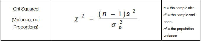
Where the number of samples is n, and the sample variance is s². The Chi-square distribution is right-skewed, especially with fewer degrees of freedom. As the degrees of freedom increase, the distribution becomes more symmetric and approaches a normal shape.

Chi-Square Variance Test

If you’re working with a single population and want to test whether its variance has changed, the Chi-Square test for variance is the right tool. It’s commonly used in Six Sigma to check whether process variation is still within acceptable limits — or if something’s gone off track.

This test compares a sample variance to a known or historical population variance using the chi-square distribution. Depending on your hypothesis, you’ll use a right-tailed, left-tailed, or two-tailed version of the test to detect increases, decreases, or any change in variation.

See the full guide: Chi-Square Test for Variance here.

Chi-Square Sample Size

Chi-square tests are susceptible to changes in the sample size. If the sample size is larger, the absolute differences become a smaller and smaller proportion of the expected value. In other words, a strong association may not come up if the sample size is small and the findings are not significant, even though they are statistically significant.

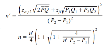
Where…

• n is sample size with correction
• n’ is sample size without continuity correction
• P₁ and P₂ are the proportions in each group
• Q₁ =1-P₁
• P̅ = P₁+P₂/2

Chi-Square Videos

https://youtu.be/EA4P1eRdEhA

https://www.youtube.com/watch?v=53kYOOr5Yhk

Additional Chi Square Examples and Helpful Links:

Chi-Square Tables

• National Institute of Standards and Technology
• Nice Chi-Square one-pager from Richland Community College
• https://people.richland.edu/james/lecture/m170/tbl-chi.html
• https://www.statisticshowto.datasciencecentral.com/tables/chi-squared-table-right-tail/
• https://www.socscistatistics.com/tests/chisquare2/default2.aspx

Chi-Square Sample Size Calculation

• https://stats.stackexchange.com/questions/340291/estimate-sample-size-for-chi-squared-test
• http://www.statskingdom.com/sample_size_chi2.html

Other Uses of Chi-Square

• Chi-Square test for goodness of fit: It is a statistical hypothesis test to see how well sample data fit into population characteristics.
• Chi-Square contingency table.

Six Sigma Black Belt Certification Chi-Square Questions:

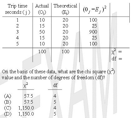
Question: The time for a fail-safe device to trip is thought to be a discrete uniform distribution from 1 to 5 seconds. To test this hypothesis, 100 tests are conducted, with results as shown below.

Based on this data, what are the Chi-Square (c2) value and the number of degrees of freedom (df)?

(A) (c2) value = 57.5, degrees of freedom = 4
(B) (c2) value = 57.5, degrees of freedom = 5
(C) (c2) value = 1,150.0, degrees of freedom = 4
(D) (c2) value = 1,150.0, degrees of freedom = 5

Answer: 

When you’re ready, there are a few ways I can help:

First, join 30,000+ other Six Sigma professionals by subscribing to my email newsletter. A short read every Monday to start your work week off correctly. Always free.

—

If you’re looking to pass your Six Sigma Green Belt or Black Belt exams, I’d recommend starting with my affordable study guide:

1)→ 🟢Pass Your Six Sigma Green Belt​​

2)→ ⚫Pass Your Six Sigma Black Belt ​​​

You’ve spent so much effort learning Lean Six Sigma. Why leave passing your certification exam up to chance? This comprehensive study guide offers 1,000+ exam-like questions for Green Belts (2,000+ for Black Belts) with full answer walkthroughs, access to instructors, detailed study material, and more.

​ Join 10,000+ students here.