Chi-Square Variance Test

Chi-Square Variance Test: The Definitive Guide for Six Sigma Practitioners

The chi-square variance test is an essential statistical tool in the Six Sigma toolkit, used to test hypotheses about the variability of a process. Whether you are verifying a supplier’s claim, evaluating the impact of a process improvement, or assessing consistency, understanding how to apply this test with confidence is key to data-driven decision-making.

What is the Chi-Square Variance Test?

The chi-square variance test determines whether the variance (or standard deviation) of a single population equals a specified value. It’s most often applied:

• In the Measure phase of DMAIC to validate baseline variability.
• In the Improve phase to confirm that changes led to reduced variation.

This test assumes that the data come from a normally distributed population. The chi-square variance test is sensitive to deviations from normality. If the data are not normally distributed, the test results may not be valid. Consider running tests for normality before applying the chi-square variance test.

To compare the variances of two groups with normal data, use the F-test. For non-normal data, use Levene’s test (or its Brown-Forsythe version) instead, because the F-test is just as sensitive to non-normality as the chi-square variance test.

When and Why to Use This Test in Six Sigma

Use the chi-square variance test when:

• You need to verify that a process’s variability meets a target or claim.
• You want to determine if an improvement effort has reduced variation.
• You’re evaluating the stability of a supplier’s product quality.

Real-World Example: A supplier claims that part diameters have a standard deviation of 1 mm. You can sample the parts, compute the sample variance, and test the claim using this test.

Hypotheses for the Chi-Square Variance Test

There are three typical forms:

1. Two-tailed test:
   • H₀: σ² = σ₀²
   • H₁: σ² ≠ σ₀² (variance is different)
2. Right-tailed test:
   • H₀: σ² ≤ σ₀²
   • H₁: σ² > σ₀² (variance is greater)
3. Left-tailed test:
   • H₀: σ² ≥ σ₀²
   • H₁: σ² < σ₀² (variance is smaller)

Test Statistic and Formula

The chi-square statistic is calculated as:

Chi-square formula:

χ² = ((n – 1) × s²) / σ₀²

Where:

• n = sample size
• s² = sample variance
• σ₀² = hypothesized population variance

Remember, Degrees of freedom (df) are calculated as the sample size minus one (df = n – 1).

This statistic follows the chi-square distribution if the population is normally distributed.

Steps to Perform the Chi-Square Variance Test

1. State the hypotheses.
2. Set the significance level (commonly α = 0.05).
3. Collect the sample and compute the sample variance.
4. Calculate the chi-square statistic.
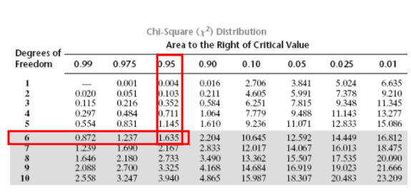
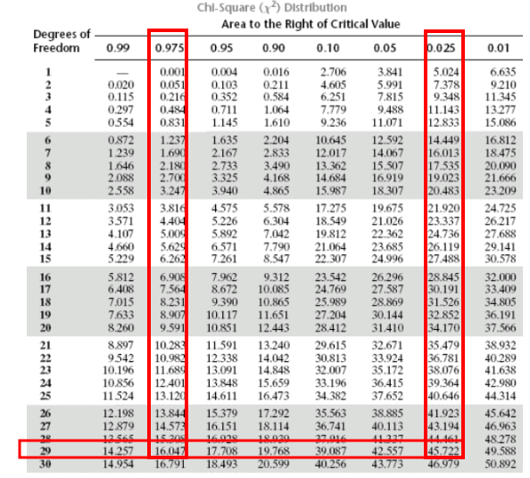
5. Determine critical value(s) from the chi-square distribution table.
   • Critical values are derived from the chi-square distribution table based on the chosen significance level (α) and degrees of freedom.
   • For instance: “At a 95% confidence level and df = 6, the critical value is 12.592.
6. Make the decision:
   • Right-tailed: Reject H₀ if test statistic > critical value.
   • Left-tailed: Reject H₀ if test statistic < critical value.
   • Two-tailed: Reject H₀ if test statistic < lower bound or > upper bound.
7. Interpret the result in context.

Practical Examples

Example 1: Reduction in Waiting Time Variation

Scenario: A bank shifts from a single queue to multiple lines to reduce waiting time variability.

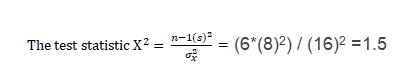
The standard deviation of customer waiting times with a single queue is 16 minutes. Accordingly, the population variance is 256 (the standard deviation squared). A sample of seven customers in the separate queues has a standard deviation of 8 minutes. Thus, the sample variance is 64 (square of the standard deviation). Test at the 5% significance level whether the variation in wait time has dropped.

The Null Hypothesis is H₀: σ₁² ≥ (16)²

The Alternative Hypothesis is H₁: σ₁² < (16)²

Let’s look at the Chi-Square table. This is a left-tailed test because the bank wants to show that variation dropped (H1: σ² < 256). df = 7 – 1 = 6. The critical value for 95% confidence is 1.63.

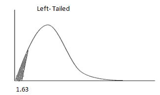
The test statistic (1.5) is less than the critical value (1.63) and is in the rejection region. Hence, the null hypothesis must be rejected. The variation in wait time decreased with the separate lines.

Example 2: Testing a Claim About Product Reliability Variance

The Barnes Company makes a DVD player and claims that the mean number of hours of use before repairs is 400, with a standard deviation of 10 hours.

The specified variance, therefore, is σo2 = 102 = 100 hours2. A new company’s marketing representative suspects the “before repair” variance is less than 100 hours2. To verify this, she tests nine machines and finds a sample mean of 410 hours and a standard deviation of 5.5. Is the sample variance significantly less than the currently claimed variance? Use α = 0.05.

In text: χ² = (n – 1) × s² / σ₀² = 8 × 5.5² / 10² = 8 × 30.25 / 100 = 2.42. Left-tailed test, df = 8, α = 0.05: critical value 2.733. Since 2.42 < 2.733, reject H₀. The sample variance is significantly less than 100 hours². (Ignore the yellow cell in the spreadsheet that ends “so fail”. The statistic is below the critical value, so H₀ is rejected, as the note under it says.)

Example 3: Investigating an Increase in Battery Life Variation

A smartwatch manufacturer receives complaints about the XYZ model’s battery life. The previous model had a known standard deviation of 7 hours (i.e., variance = 49). The company tests 11 new units and finds a sample standard deviation of 9 hours (variance = 81). They want to determine whether the new model has significantly more variability in battery life.

Hypotheses:

• H₀: σ² ≤ 49
• H₁: σ² > 49 (right-tailed test)

Step 1: Compute Test Statistic

χ² = ((n – 1) × s²) / σ₀² = (10 × 81) / 49 = 16.53

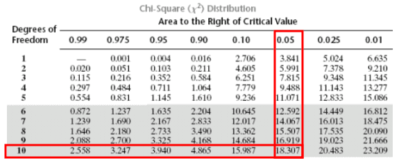
Step 2: Determine Critical Value

• Degrees of freedom = 11 – 1 = 10
• At α = 0.05 (right-tail), critical value = 18.307

Step 3: Decision

Since 16.53 < 18.307, we fail to reject the null hypothesis. There’s insufficient evidence to claim the new smartwatch has increased battery life variation.

📊 See visual reference:

• 
• 

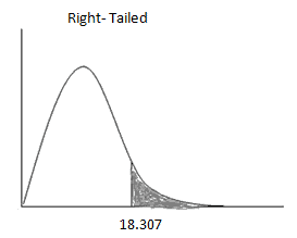
✅ Tip: This is a right-tailed test because the company wants proof of increased variability. The tail comes from the question asked, not from which way the sample came out.

Example 4: Comparing Wage Variability Across Teams (Two-Tailed Test)

HR suspects that the new Digital Technology team’s wages have different variability than the established Java Technology team. Historically, the Java team has had a standard deviation of $49K, or a variance of 2,401. A sample of 30 Digital team employees shows a standard deviation of $70K, or a variance of 4,900.

We want to test whether this difference is statistically significant.

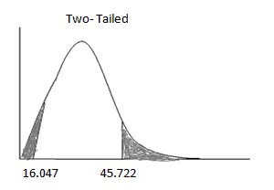
Hypotheses:

• H₀: σ² = 2,401
• H₁: σ² ≠ 2,401 (two-tailed test)

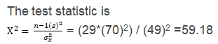
Step 1: Compute Test Statistic

χ² = ((n – 1) × s²) / σ₀² = (29 × 4,900) / 2,401 = 59.18

Step 2: Determine Critical Values

• Degrees of freedom = 30 – 1 = 29
• Left-tail (α/2 = 0.025): Critical value = 16.047
• Right-tail (α/2 = 0.025): Critical value = 45.722

Step 3: Decision

Since 59.18 > 45.722, the test statistic lies in the right rejection region.
We reject the null hypothesis: there is significant evidence that the wage variation in the new team is different from the Java team.

📊 Visual references:

• 
• 
• 

Reminder: In a two-tailed test, we split the alpha level (α) between both ends of the distribution. Use:

• α/2 for each tail
• For the left-tail critical value, use the (1 − α/2) column of a right-tail table. That point has a cumulative (left-tail) probability of α/2.

Summary Table of Tail Types

Special Cases and Considerations

• Normality Assumption: The test relies on normal distribution. Use histograms or normality tests to validate.
• Sample Size Sensitivity: Small samples may not adequately reflect the population. Consider larger n when feasible.
• Tail Direction Confusion: Students often misinterpret whether a test should be right- or left-tailed. A simple rule:
  • If you want to show the variance decreased (H₁: σ² < σ₀²), it’s a left-tailed test
  • If you want to show the variance increased (H₁: σ² > σ₀²), it’s a right-tailed test

Chi-Square Table Usage

• Tables typically provide right-tail critical values.
• For left-tail tests, use the (1 – α) column, for example the 0.95 column when α = 0.05.
• For two-tailed tests, use α/2 in both tails.

Conclusion

The chi-square variance test provides a rigorous method for assessing process variation in a single population. It is a vital tool for Green and Black Belts during Measure and Improve phases of DMAIC. Proper application ensures improvements are statistically significant and aligned with Six Sigma principles of reducing variability and enhancing quality.

When you’re ready, there are a few ways I can help:

First, join 12,000+ other Six Sigma professionals by subscribing to my email newsletter. A short read every Monday to start your work week off correctly. Always free.

* * *

If you’re looking to pass your Six Sigma Yellow Belt, Green Belt or Black Belt exam, I’d recommend starting with my affordable study guide:

1)→ 🟡Pass Your Six Sigma Yellow Belt: built for ASQ, IASSC and ILSSI, 1,700+ practice questions with explanations, and six full-length mock exams for your exam

2)→ 🟢Pass Your Six Sigma Green Belt: a study guide organized by the exam Body of Knowledge, 1,000+ practice questions with detailed answer explanations, and 15+ full-length mock exams

3)→ ⚫Pass Your Six Sigma Black Belt: the full Black Belt Body of Knowledge, 2,000+ practice questions with detailed answer explanations, and 15+ full-length mock exams

You’ve spent so much effort learning Lean Six Sigma. Why leave passing your certification exam up to chance? This comprehensive study guide offers 1,700+ exam-like questions for Yellow Belts, 1,000+ for Green Belts and 2,000+ for Black Belts with full answer walkthroughs, access to instructors, detailed study material, and more.

​ Thousands have used this system to prepare. Join them here.