The chi-square test of independence (also called a chi-square test of association) determines whether two categorical variables are statistically independent of each other.
In Six Sigma, this is extremely useful for analyzing contingency tables. For example, you might want to see if defect occurrence is independent of the shift, or if customer satisfaction ratings are independent of location. It helps answer questions like, “Are these two factors related, or are any differences just random variation?”
When to use: Use a chi-square test of independence in the Analyze phase when you have counts of outcomes classified by two categorical factors and you suspect there may be a relationship. For instance, you collected data on defects categorized by machine and defect type – is the pattern of defect types the same for each machine (independence), or does one machine have disproportionately more of certain defects (dependence)? Another example: a call center manager might check if call resolution outcome is independent of the agent’s experience level. Essentially, whenever you have an R×C table of counts (R rows = categories of variable1, C columns = categories of variable2), this test can tell you if there’s an association.
Hypotheses:
- H₀: The two categorical variables are independent (no association). In other words, the distribution of one variable is the same for all categories of the other variable.
- H₁: The two variables are not independent (there is an association). At least some categories of one variable are linked to differences in the distribution of the other.
Assumptions: Similar to the GOF test, the observations should be independent of each other, and sample size should be sufficiently large (expected counts ideally ≥ 5 in each cell of the table, or at least in the vast majority of cells). If any cell has an expected count too low, results may not be reliable (you might combine sparse categories or use Fisher’s exact test for a 2×2 table if necessary).
The data for an independence test are typically arranged in a contingency tablesixsigmastudyguide.com. Each cell of the table contains the count of observations that fall into the corresponding row category and column category combination. For example, rows might be “Machine A vs Machine B” and columns “Defect Type X, Y, Z,” with each cell showing how many defects of each type occurred on each machine.
Steps to Perform a Chi-Square Test of Independence
- Set up hypotheses:
- Null (H₀): The two variables are independent (no association between them).
- Alternative (H₁): The two variables are associated (the distribution of one depends on the other).
- Choose significance level (α): Often 0.05.
- Create the contingency table of observed counts: Organize your data into a table of r rows and c columns. Calculate the row totals, column totals, and the grand total n. These totals are needed to compute expected counts.
- Calculate expected counts for each cell: If H₀ is true (independence), the expected frequency in a cell is:
Eij=(Row i total)×(Column j total)n.E_{ij} = \frac{(\text{Row i total}) \times (\text{Column j total})}{n}.Eij=n(Row i total)×(Column j total).
This comes from probability theory – if events are independent, P(row i and col j) = P(row i)*P(col j), so expected count = (row proportion * column proportion * n). You do this for every cellsixsigmastudyguide.com. For example, if in a survey 60% of responses were from Region A (row) and 30% preferred Product X (column), then under independence you’d expect 0.6 * 0.3 = 18% of total respondents to fall in (Region A, Product X) cell. - Compute the chi-square statistic: Sum over all cells:
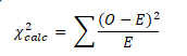
χ2=∑i=1r∑j=1c(Oij−Eij)2Eij.\chi^2 = \sum_{i=1}^{r}\sum_{j=1}^{c} \frac{(O_{ij} – E_{ij})^2}{E_{ij}}.χ2=∑i=1r∑j=1cEij(Oij−Eij)2.
Each cell’s contribution is calculated similarly to the GOF test, comparing observed vs expectedsimplilearn.comsimplilearn.com. - Degrees of freedom: df = (number of rows – 1) × (number of columns – 1)simplilearn.com. This formula reflects that once you know all the row and column totals, only that many cells are free to vary independently; the rest are determined by totals.
- Find the critical value (right-tailed): Use the χ² table for the given df at your α. This test is right-tailed – large χ² means observed counts diverge from expected (indicating dependence). Alternatively, calculate the p-value corresponding to the χ² statistic and df.
- Conclusion: If χ²_stat > χ²_critical (p < α), reject H₀. Conclude there is a significant association between the two variables – the differences in the contingency table are unlikely due to chance. If χ²_stat is not beyond critical (p ≥ α), fail to reject H₀, meaning you do not have evidence of an association (the variables could be independent).
Independence Test Example: Process Defects by Shift
As a Six Sigma example, suppose a manufacturing team wants to know if the occurrence of defect types is independent of the production shift (Day shift vs. Night shift). They categorize defects into three types: Type A, Type B, Type C. Over a month, they collect the following data:
- Day Shift: 16 defects of Type A, 4 of Type B, 10 of Type C (Total = 30 defects in day shift).
- Night Shift: 8 defects of Type A, 12 of Type B, 10 of Type C (Total = 30 defects in night shift).
(Total defects observed = 60.)
The contingency table of observed counts would be:
| Type A | Type B | Type C | Row Total | |
|---|---|---|---|---|
| Day Shift | 16 | 4 | 10 | 30 |
| Night Shift | 8 | 12 | 10 | 30 |
| Col Total | 24 | 16 | 20 | 60 |
We’ll test at 95% confidence (α = 0.05) if shift and defect type are independent.
Step 1 – Hypotheses:
H₀: Defect type is independent of shift (no relationship between shift and defect distribution).
H₁: Defect type depends on shift (the pattern of defect types differs between day and night shifts).
Step 2 – Significance: α = 0.05.
Step 3 – Observed data: (as in the table above).
Step 4 – Expected counts: Compute for each cell using E = (row total * col total) / grand total. For example:
- Expected in Day Shift, Type A = (Day total 30 * Type A total 24) / 60 = 12.
- Expected in Day, Type B = (30 * 16) / 60 = 8.
- Expected in Day, Type C = (30 * 20) / 60 = 10.
- Expected in Night, Type A = (30 * 24) / 60 = 12.
- Expected in Night, Type B = (30 * 16) / 60 = 8.
- Expected in Night, Type C = (30 * 20) / 60 = 10.
So the expected table (under H₀) would be:
| Type A | Type B | Type C | Row Total | |
|---|---|---|---|---|
| Day (Exp) | 12 | 8 | 10 | 30 |
| Night (Exp) | 12 | 8 | 10 | 30 |
| Col Total | 24 | 16 | 20 | 60 |
Step 5 – χ² calculation: Sum (O−E)²/E for all 6 cells:
- Day/A: (16−12)²/12 = (4)²/12 = 16/12 = 1.33
- Day/B: (4−8)²/8 = (−4)²/8 = 16/8 = 2.00
- Day/C: (10−10)²/10 = 0
- Night/A: (8−12)²/12 = (−4)²/12 = 16/12 = 1.33
- Night/B: (12−8)²/8 = (4)²/8 = 16/8 = 2.00
- Night/C: (10−10)²/10 = 0
χ²_stat = 1.33 + 2.00 + 0 + 1.33 + 2.00 + 0 = 6.67 (approximately).
Step 6 – Degrees of freedom: df = (2–1)*(3–1) = 1 * 2 = 2.
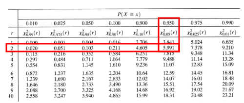
Step 7 – Critical value: For df = 2 and α = 0.05 (right-tailed), χ²_critical = 5.991sixsigmastudyguide.com.
Step 8 – Conclusion: Our χ²_stat = 6.67 which is greater than 5.991. That means p-value < 0.05. We reject H₀ and conclude there is a significant association between shift and defect type. In practical terms, the mix of defect types is different on day vs. night shift. Looking at the observed vs expected, Day shift had more Type A than expected and fewer Type B, whereas Night shift had more Type B and fewer Type A than expected. This insight suggests that shift (perhaps the conditions or personnel on each shift) has an impact on what kinds of defects occur. That information can guide further root cause analysis (maybe day shift has an issue causing Type A defects, while night shift struggles with Type B).
(Note: If our χ²_stat had been less than 5.991, we’d conclude there’s no evidence of a difference – the defect pattern could be essentially the same on both shifts.)
This example demonstrates how the chi-square test of independence helps identify relationships between categorical factors in a process. In a Six Sigma project, such a finding would prompt investigation into why the association exists (e.g., do day and night shifts follow different procedures or have different skill levels leading to certain defects?). It’s a powerful Analyze phase tool for validating or disproving suspected factor-effect relationships.
(In this test, as with GOF, we used the right tail of the χ² distribution. A large χ² (here ~6.67) beyond the cutoff signaled a significant difference. Independence tests are always right-tailed because only greater divergence (not a deficiency) indicates dependence.)
The Chi-Square Test of Independence determines whether there is an association between two categorical variables (like gender and course choice). For example, the Chi-Square Test of Independence examines the association between one category, like gender (male and female), and another category, like the percentage of absenteeism in a school. The Chi-Square Test of Independence is a non-parametric test. In other words, you do not need to assume a normal distribution to perform the test.
A Chi-Square test uses a contingency table to analyze the data. Each row shows the categories of one variable. Similarly, each column shows the categories of another variable. Each variable must have two or more categories. Each cell reflects the total number of cases for a specific pair of categories.
Assumptions of Chi-Square Test of Independence
- Variables must be nominal or categorical
- Categories of variables are mutually exclusive
- The sampling method is a simple random sampling
- The data in the contingency table are frequencies or count
Steps to Perform Chi-Square Test of Independence
Step1: Define the Null Hypothesis and Alternative Hypothesis
- Null Hypothesis (H0): There is no association between two categorical variables
- Alternative Hypothesis (H1): There is a significant association between two categorical variables
Step2: Specify the level of significance
Step 3: Compute χ2 statistic
- O is the observed frequency
- E is the expected frequency
The expected frequency is calculated for each cell = (frequency of columns * frequency of rows)/ n
Step 4: Calculate the degree of freedom = (number of rows -) * (number of columns -1)= (r-1) * (c-1)
Step 5: Find the critical value based on degrees of freedom
Step 6: Finally, draw the statistical conclusion: If the test statistic value is greater than the critical value, reject the null hypothesis, and hence, we can conclude that there is a significant association between two categorical variables.
Chi-Square Test of Independence Example
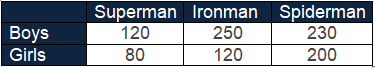
For example, 1000 middle school students are asked which their favorite superhero is: Superman, Ironman, or Spiderman. At a 95% confidence level, would you conclude that there is a relationship between gender and superhero characters?
- Null Hypothesis (H0): There is no association between gender and favorite superhero characters.
- Alternative Hypothesis (H1): There is a significant association between gender and favorite superhero characters.
Level of significance: α=0.05:
First, calculate the expected frequency:
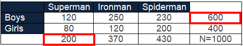
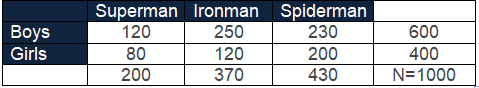
For the cell (Boys, Superman) = (200 * 600)/ 1000 = 120
Similarly, determine the expected frequency of all cells:
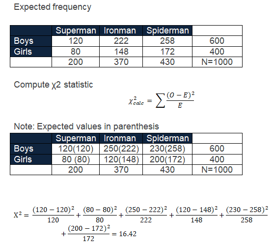
Degrees of freedom = (r – 1) * (c – 1) = (2 – 1) * (3 – 1) =2
Chi-Square critical value for 2 degrees of freedom =5.991
The test statistic value is greater than the critical value; hence, we can reject the null hypothesis.
So, we can deduce a significant association between gender and favorite superhero characters.
Download Chi-Square Test of Independence Excel Exemplar
When you’re ready, there are a few ways I can help:
First, join 30,000+ other Six Sigma professionals by subscribing to my email newsletter. A short read every Monday to start your work week off correctly. Always free.
—
If you’re looking to pass your Six Sigma Green Belt or Black Belt exams, I’d recommend starting with my affordable study guide:
1)→ 🟢Pass Your Six Sigma Green Belt
2)→ ⚫Pass Your Six Sigma Black Belt
You’ve spent so much effort learning Lean Six Sigma. Why leave passing your certification exam up to chance? This comprehensive study guide offers 1,000+ exam-like questions for Green Belts (2,000+ for Black Belts) with full answer walkthroughs, access to instructors, detailed study material, and more.