Response surface modeling, also known as the response surface method, is a mathematical and statistical technique useful for developing, improving, and optimizing the process. The response surface method is useful for analyzing the problem when several independent variables (also known as predictor variables) influence the dependent variable or response. In short Response Surface Method is denoted as RSM.

Use Response Surface modeling to hit a certain target, reduce variability in a process, maximize or minimize a response, make a process more robust despite uncontrollable noise, and even pursue multiple goals.

Example: A researcher estimating the effects of independent variables like temperature and pressure influences the yield.

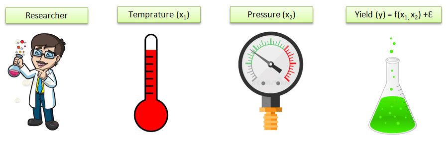
The assumptions of independent variables are continuous and can be controllable by the experimenter. Similarly, the response variable is assumed to be a random variable.

Purpose of Response Surface Modeling

• To find optimal or improved settings
• Analyze and rectify process problems and weak points
• Robust the process or product against the external influences

When to use RSM

Taguchi or full factorial design is the best option when only a few factors influence the design. Whereas, the response surface method is useful when several factors influence the response or design. The application of RSM is in various fields and industries, primarily agricultural, pharmaceutical, and electronic fields. However, the main objective of RSM is to optimize the response.

How to conduct Response Surface Modeling

• The independent variables x₁, x₂,x₃…x_k in RSM, and the assumption is that response is a function of a set of independent variables. While the function can be represented in some regions of the polynomial model.

y= f(x_i)

y= f(x₁, x₂,x₃…x_k) 

y is the response or dependent variable and k independent variable.

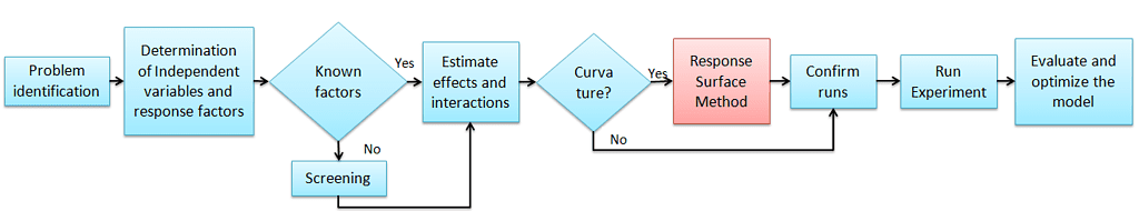
• If the factors are known, directly estimate the effects and also the interactions. Otherwise, use a screening method to calculate the unknown factors.

Estimate the interaction effect using the 1^st order model.

y= β₀+β₁x₁+ β₂x₂+ Ɛ

Ɛ-Error

β₀, β_1, β₂ are the constants.

• If the curvature exists, then use RSM. Use 2^nd order model to approximate the response variable.

y= β₀+β₁x₁+ β₂x₂+ β₁₂x₁ x₂+ β₁₁x₁²+ β₂₂x₂²+ Ɛ

• Finally, plot the graph and identify the stationary point. Maximum, minimum response or saddle point, which is the sudden drastic change between minimum to the maximum from the values X₁, X₂, X₃…

Example of Response Surface Modeling

Example: A researcher wants to install air-conditioning in a room, and they are estimating the efficiency of the room. The efficiency of the room depends upon the temperature as well as the volume of the room.

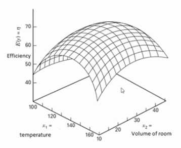
For instance, If the volume increases, temperature increases; hence efficiency decreases. From the above graph, it is clear that the top of the surface indicates high efficiency, and also efficiency is low (45) at high temperatures (160 degrees). The aim is to move specifically toward the top of the surface. Moreover, this can be justified with a mathematical equation like a first-order polynomial, second-order polynomial, etc.,

Different methods of RSM

RSM is often a sequential procedure when we are at a point on the response surface that is remote from the optimum. Thus in this method, move rapidly from the current point to the optimum point (sources are minimum, but the output is maximum) with a sequence.

There are basically two methods of RSM to obtain the optimum point.

• The method of steepest ascent
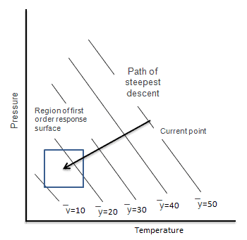
• The method of steepest descent

Method of Steepest Ascent: It is a process of moving sequentially toward the maximum increase in the response to the optimum response.

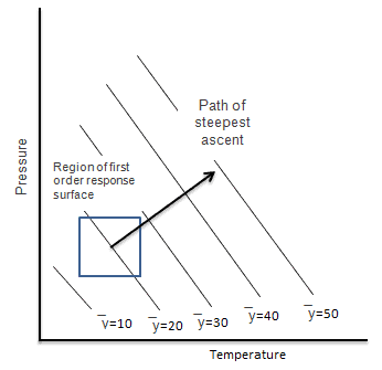
Method of steepest descent: Use the method of steepest descent to minimize the response. To move from the current position ̅y=50 to ̅y =10 in a faster way, use the method of steepest descent.

Types of Response Surface Modeling

• Central composite Design (CCD)
• Box-Behnken Design (BBD)

Central composite design (CCD)

The central composite design is the most popular and flexible response surface design, and most researchers prefer this design. Box and Wison first published a central composite design in 1951.

A central composite design always will have 2 levels and k influencing factors. It consists of center points as well as axial points. First of all, create a 2^k factorial or a 2k-p fractional factorial design, and then append a set of extra runs referred to as axial points (also known as star points).

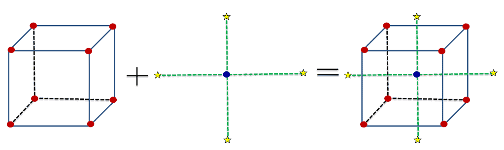
The 2^k and 2^k-p portion of the design allows us to fit first-order terms and interactions. Likewise, the axial points supply the extra level required to fit the second-order model.

Box-Behnken Design (BBD)

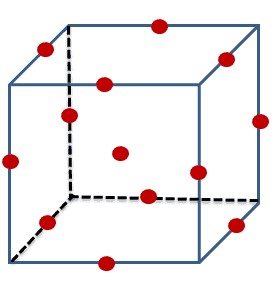
Box-Behnken Design (BBD) is the popular response surface method for a three-level factor to fit the second-order model to the response. Box and Behnken first developed this in 1960.

Box-Behnken Design is a combination of two-level factorial designs with incomplete block designs. The main advantage of Box–Behnken design is it does not contain any points at the extremes of the cubic region created by the two-level factorial level combinations. In other words, no corner points.

The key difference between Taguchi and Response surface methodology

Response Surface Modeling Important Videos